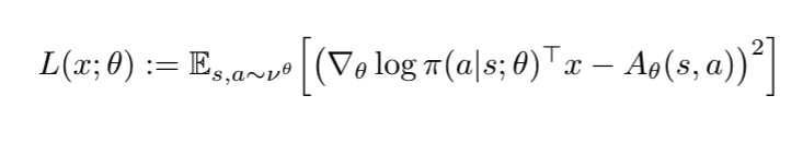
I’m relatively new to Pytorch and am trying to implement a natural actor-critic (NAC) algorithm where my policy pi is a DNN. See algorithm 2 in Thomas (2014) for a simple example. In order to do this, I want to compute the natural gradient x by minimising the following loss, where nu is the on-policy state-action distribution, and A is the advantage function (which I already have):
My question is: How do I best (most efficiently) compute the score function (the derivative of the log of the policy w.r.t. its parameters theta)?
I have a naive implementation already, but it involves computing this score function for each individual state-action sample using a single application of torch.autograd.grad, and is therefore horrendously slow. I am aware that NAC algorithms have been used before for fairly high-dimensional control tasks, but have been unable to find an existing implementation online.
Hi Thomas, thanks very much for your reply! I’m already sampling mini-batches (of size 32) from my replay buffer but this is still incredibly slow (even though I’m only using a toy environment at the moment). Perhaps to make things more concrete, my (pseudo-ish) code for computing the scores is as follows:
scores = []

log_probs = self.policy(states).log_prob(actions)

for params in self.actor.parameters():
    scores.append(torch.stack([torch.autograd.grad(outputs=l_p, inputs=params, retain_graph=True)[0] for l_p in log_probs]))
It may well be that this is the only/fastest way of doing things (although I doubt that!), but in which case I suppose I just need to perform this computation as few times as I possible can during learning.
Any further suggestions or comments are greatly appreciated
If you have a sizeable network, I think taking the loop over the parameters as the outer loop is very likely worse than the other way round and taking the gradients of every parameter in one go even if you then need to disentangle them.
The other question is whether you really need the scores separately or are later doing something that would lend itself to rewriting as a single loss to take the gradient of.
Hi Thomas, thanks again for the input. In reply to your two points:
Thanks, this was left over from a previous version of the function and is an unecessary loop, I will remove it
This would be the ideal way forward, I agree, and I have been search for a solution in this direction. Unfortunately I haven’t been able to rewrite the expectation of a loss function (such as the squared error between terms in the expression in my original post above) as a loss function applied to an expectation. In the most general case, Jensen’s inequality of course tells us that (when using a convex loss function) the latter term will be less than or equal to the first, and so bounding the latter gives no guarantee on bounding the former, although it maybe the case that there is a trick to get round this here?
I realise this is diving a little more into the maths than the Pytorch implementation at this point, but I’m not so experienced with translating the first into the second, so I could definitely be missing some obvious things here!
Well, so outside RL this outer expectation is usually covered by minibatching + the iteration. Just like Algorithm 2 in the reference seems to suggest that a single a_t, s_t+1 pair is sampled in line 7.
Of course, the usual thing is to do something that is vaguely linear in the gradient, so it might not be applicable.
What is the exact maths that you’re trying to translate?
That makes sense. To be more concrete about my implementation: I’m running my agent, storing each state, action, reward, etc. tuple in a replay buffer, then after each episode sampling a mini-batch of 32 (a somewhat arbitrary choice) such tuples to compute the terms inside the expectation in the image above, then backpropagating to minimise the loss L. The parameters theta are then updated on a slower timescale (or outer loop) using x.
My understanding is that the Thomas (2014) pseudocode in algorithm 2 effectively uses a mini-batch of size one at every time-step, though with a large number of time-steps this seems like it would be less efficient than my current implementation? For reference/clarity, line 13 in Thomas (2014) contains the update that I am struggling with, where the author uses w instead of x, and also uses eligibility traces e (other than that it can be seen that the gradient update is simply that of L as given above).
The exact maths is only the loss function above and the related pseudocode/derivation in Thomas (2014), so not really that advanced! I suppose my issue is that something that seems so mathematically simple is so slow in my implementation, but this could be because I’m not appreciating some of the subtleties of Pytorch and automatic differentiation more generally.
So if I understand you correctly, you minibatch s and a in line 4 and 7 but take the time steps individually? But then you might be able to just take a single w and v by summing the terms in delta terms in 13 + 14 and the sum the log before the differentiation.
If you combine several timesteps, you’d get slower updates of things, I would not know if that is too much…
Essentially yes, a single datum (state, action, reward, etc.) is collected at each time step t and stored in the buffer. Summing over terms then manually computing the gradient update to x (as opposed to forming the loss function explicitly and then backpropagating) might be the answer though; I hadn’t considered that! Thanks very much, I’ll try this out and see how I get on