I know this isn’t about PyTorch but if anyone would be able to help with weights updates in almost pure Python code for MLP on XOR, that’ll be helpful to understand backprop and autograd eventually! Thanks in advance. Sorry again for cross-posting.
Given the XOR problem:
X = xor_input = np.array([[0,0], [0,1], [1,0], [1,1]])
Y = xor_output = np.array([[0,1,1,0]]).T
And a simple
- two layered Multi-Layered Perceptron (MLP) with
- sigmoid activations between them and
- Mean Square Error (MSE) as the loss function/optimization criterion
[code]:
def sigmoid(x): # Returns values that sums to one.
    return 1 / (1 + np.exp(-x))

def sigmoid_derivative(sx): # For backpropagation.
    # See https://math.stackexchange.com/a/1225116
    return sx * (1 - sx)

# Cost functions.
def mse(predicted, truth):
    return np.sum(np.square(truth - predicted))

X = xor_input = np.array([[0,0], [0,1], [1,0], [1,1]])
Y = xor_output = np.array([[0,1,1,0]]).T

# Define the shape of the weight vector.
num_data, input_dim = X.shape
# Lets set the dimensions for the intermediate layer.
hidden_dim = 5
# Initialize weights between the input layers and the hidden layer.
W1 = np.random.random((input_dim, hidden_dim))

# Define the shape of the output vector.
output_dim = len(Y.T)
# Initialize weights between the hidden layers and the output layer.
W2 = np.random.random((hidden_dim, output_dim))
And given the stopping criteria as a fixed no. of epochs (no. of iterations through the X and Y) with a fixed learning rate of 0.3:
# Initialize weigh
num_epochs = 10000
learning_rate = 0.3
When I run through the forward-backward propagation and update the weights in each epoch, how should I update the weights?
I tried to simply add the product of the learning rate with the dot product of the backpropagated derivative with the layer outputs but the model still only updated the weights in one direction causing all the weights to degrade to near zero.
for epoch_n in range(num_epochs):
    layer0 = X
    # Forward propagation.

    # Inside the perceptron, Step 2.
    layer1 = sigmoid(np.dot(layer0, W1))
    layer2 = sigmoid(np.dot(layer1, W2))

    # Back propagation (Y -> layer2)

    # How much did we miss in the predictions?
    layer2_error = mse(layer2, Y)

    #print(layer2_error)
    # In what direction is the target value?
    # Were we really close? If so, don't change too much.
    layer2_delta = layer2_error * sigmoid_derivative(layer2)

    # Back propagation (layer2 -> layer1)
    # How much did each layer1 value contribute to the layer2 error (according to the weights)?
    layer1_error = np.dot(layer2_delta, W2.T)
    layer1_delta = layer1_error * sigmoid_derivative(layer1)

    # update weights
    W2 += - learning_rate * np.dot(layer1.T, layer2_delta)
    W1 += - learning_rate * np.dot(layer0.T, layer1_delta)
    #print(np.dot(layer0.T, layer1_delta))
    #print(epoch_n, list((layer2)))

    # Log the loss value as we proceed through the epochs.
    losses.append(layer2_error.mean())
How should the weights be updated correctly?
Full code:
from itertools import chain
import matplotlib.pyplot as plt
import numpy as np
np.random.seed(0)
def sigmoid(x): # Returns values that sums to one.
return 1 / (1 + np.exp(-x))
def sigmoid_derivative(sx):
# See https://math.stackexchange.com/a/1225116
return sx * (1 - sx)
# Cost functions.
def mse(predicted, truth):
return np.sum(np.square(truth - predicted))
X = xor_input = np.array([[0,0], [0,1], [1,0], [1,1]])
Y = xor_output = np.array([[0,1,1,0]]).T
# Define the shape of the weight vector.
num_data, input_dim = X.shape
# Lets set the dimensions for the intermediate layer.
hidden_dim = 5
# Initialize weights between the input layers and the hidden layer.
W1 = np.random.random((input_dim, hidden_dim))
# Define the shape of the output vector.
output_dim = len(Y.T)
# Initialize weights between the hidden layers and the output layer.
W2 = np.random.random((hidden_dim, output_dim))
# Initialize weigh
num_epochs = 10000
learning_rate = 0.3
losses = []
for epoch_n in range(num_epochs):
layer0 = X
# Forward propagation.
# Inside the perceptron, Step 2.
layer1 = sigmoid(np.dot(layer0, W1))
layer2 = sigmoid(np.dot(layer1, W2))
# Back propagation (Y -> layer2)
# How much did we miss in the predictions?
layer2_error = mse(layer2, Y)
#print(layer2_error)
# In what direction is the target value?
# Were we really close? If so, don't change too much.
layer2_delta = layer2_error * sigmoid_derivative(layer2)
# Back propagation (layer2 -> layer1)
# How much did each layer1 value contribute to the layer2 error (according to the weights)?
layer1_error = np.dot(layer2_delta, W2.T)
layer1_delta = layer1_error * sigmoid_derivative(layer1)
# update weights
W2 += - learning_rate * np.dot(layer1.T, layer2_delta)
W1 += - learning_rate * np.dot(layer0.T, layer1_delta)
#print(np.dot(layer0.T, layer1_delta))
#print(epoch_n, list((layer2)))
# Log the loss value as we proceed through the epochs.
losses.append(layer2_error.mean())
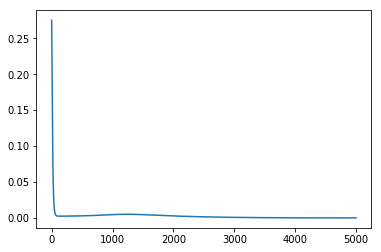
# Visualize the losses
plt.plot(losses)
plt.show()