Hi, I have a question about how to implement the universal Lagrange Multiplier and KKT conditions with PyTorch. Specificlly, the optimziation problem is
$$
\min f(x), s.t. h(x)=0, g(x)<=0
$$
Although I know the method to solve this problem but I don’t know how to implement it with PyTorch. Could you give me an example? Thank you.
Hi,
It depends which methods you want to use to solve this?
In general, there are only unconstrained, gradient descent based optimizers in pytorch as it is what can be done efficiently for neural nets.
I just want to do an optimization problem with constriants. With Lagrange Multiplier and KKT conditions, the problem could be converted to an unconstrained problem. I think this problem could be optimized with PyTorch. But there are many conditions for the lagrange multiplier, so I don’t know how to implement it. Could you give me an example? Thank you.
I don’t have an example implementation from the top of my mind.
If you have a specific algorithm in mind you might be able to find an implementation online though.
Whatever algorithm you want to use to solve your unconstrained problem, you can use pytorch to get gradients and/or perform the steps you need.
But there are many conditions for the lagrange multiplier, so I don’t know how to implement it.
Lagrage Multipliers is just one way to rewrite the problem. You still need to select an optimization algorithm to solve this new problem.
Hiiiii Sakuraiiiii!
To expand a little on what Alban has said, the problem is as follows:
If I have an optimization problem where I seek to minimize a loss
function (e.g., a neural-network training loss), but then add constraints
to it, it is true that I can use Lagrange multipliers to convert the
constrained optimization to an unconstrained optimization.
However, this unconstrained optimization problem is no longer a
minimization problem, but rather one of finding a stationary point
(also called a critical point) of the augmented loss function.
That is, the gradient (including the gradient with respect to the
Lagrange multipliers) will vanish at the stationary-point solution, but
this solution need not be a minimum (with respect to the Lagrange
multipliers).
A simple example illustrates the difference:
We can minimize x**2 with gradient descent just fine, and the minimum
occurs ar x = 0 where the derivative vanishes.
The function x**3 also has a stationary point at x = 0 (where the
derivative vanishes), but gradient descent is no good for finding it.
Once x ends up less than zero – even by a little bit – gradient descent
will keep pushing x to become more and more negative, and off to
-inf.
I don’t know enough to state that you can’t use gradient descent with
Lagrange multipliers, but I don’t know how to do it.
If I were to try to hack something together for your problem, I would
try adding penalties for constraint violation to your loss function, and
use pytorch / gradient descent to minimize that.
So you could add, for example, alpha * h(x)**2 for your equality
constraints, and beta * min (g(x), 0)**2 for your inequality
constraints. As you increase alpha and beta, minimizing your loss
function will increasing push you in the direction of satisfying your
constraints. (Perhaps abs() would be better than **2, as it avoids
the “softer” quadratic minimum.)
You could say that adding these penalties to you loss function will
“encourage” your constraints to be close to being satisfied, but it won’t
force them to be satisfied.
Good luck.
K. Frank
2 Likes
Hi, KFrank. Thank you very much. I will follow you advice. But according to what you said, I have another question that maybe I can minimize abs(\nambla L) whose minimum is 0, where L=f(x)+\lambda h(x) + \mu g(x). Is it will be worked?
Hiiiii Sakuraiiiii!
In principle, you could do this. The problem (in general, and in
the specific context of pytorch) is how are you going to calculate
abs (nabla L)?
If you can do it analytically, great. (But then you might even be able
to solve your full optimization problem analytically.)
You could imagine using pytorch’s autograd to numerically calculate
nabla L, but if you then want to use gradient descent to minimize
abs (nabla L), you will be, in effect, calculating second derivatives
of L with respect to the parameters of your model and your Lagrange
multiplier.
Research using and calculating the Hessian matrix in pytorch to
see what people have been able to do with this and the difficulties
involved.
Best.
K. Frank
You’re right. Thank you very much.
Note that here, we know w.r.t. which variables the Lagrangian would be maximized and w.r.t. which ones it would be minimized, so in this way the problem is much easier than “find a saddle point”.
Indeed, while there are few guarantees (though some papers seem to appear, in particular for convex/concave problems) an alternating optimization scheme where you take descent steps for the minimization vars and ascent steps in the maximization vars could be expected to find something (this is basically what the GAN does too in Gparam = argmin_Gparam max_Dparam E(D(x_true, x_fake)), and from there we know that balancing the two types of steps is important, more so for us because the maximization is unconstrained by construction - as it’s designed to take max = infinity for violation of the linear constraints).
For the inequality (KKT) conditions, you could probably use an active set method.
Fun fact, and here we go back to @KFrank’s advice to use penalty terms: If memory serves me well, the active-set-method of Lawson and Hanson for NNLS with linear constraints uses a 1/epsilon (“machine precision”) penalty for the equality constraints.
Best regards
Thomas
Hi Thomas!
I don’t think it is as simple as this, the reason being that at the
constrained minimum, the gradient of the loss function plus the
Lagrange-multiplier terms in the direction of the Lagrange
multiplier is flat.
Consider the trivial example:
Minimize x**2 / 2, where x = 1. To do so, we find the critical
point of x**2 / 2 + lambda * (x - 1). The critical point is
(1, -1), and at the critical point the Hessian matrix is
[[1, 1], [1, 0]]. (The second partial with respect to lambda
is indeed 0.)
Letting phi = (1 + sqrt (5)) / 2 (the so-called “golden
ratio”), the Hessian’s eigenvectors (“principal axes”) are
(phi, 1) and (1, -phi) (positive and negative curvature,
receptively). These don’t align with the original variable, x, and
the Lagrange multiplier.
Even near the constrained minimum, I don’t see how you will
know in which directions to take “descent” steps and “ascent”
steps without calculating the second partials and looking at
the Hessian matrix.
Best.
K. Frank
I could be wrong, but I think that while yes, you won’t get optimal directions for the steps (which isn’t surprising when using SGD), it would still find the right directions because the structure of the problem min_x max_lambda L says we can minimize w.r.t. x and maximize w.r.t. lambda.
lfn = lambda x, l: x**2 / 2 + l * (x - 1)
x = torch.tensor(-0.1, requires_grad=True)
l = torch.tensor(0.0, requires_grad=True)

xs = []
ls = []
for i in range(200):
    f = lfn(x, l)
    dx, dl = torch.autograd.grad(f, [x, l])
    with torch.no_grad():
        x -= 1e-1 * dx
        l += 1e-1 * dl
    xs.append(x.item())
    ls.append(l.item())

%matplotlib inline
from matplotlib import pyplot
pyplot.plot(xs)
pyplot.plot(ls)
x.item()
gives 0.9999565482139587.
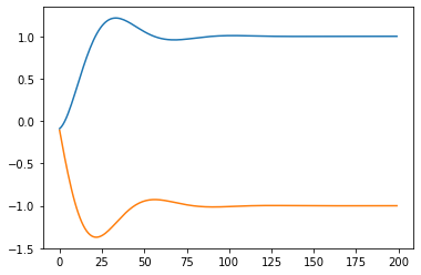
Best regards
Thomas
Hi Thomas!
Thanks, you’re right. I stand corrected.
See, for example, “Constrained Differential Optimization,” Platt
and Barr, 1988:
https://papers.nips.cc/paper/4-constrained-differential-optimization.pdf
Best.
K. Frank