I define my Dataset class:
class MyDataset(Dataset):
    def __init__(self, images, n, labels=None, transforms=None):
        self.X = images
        self.y = labels
        self.n = n
        self.transforms = transforms

    def __len__(self):
        return (len(self.X))

    def __getitem__(self, i):
        data = self.X.iloc[i, :]
#         print(data.shape)
        data = np.asarray(data).astype(np.float).reshape(1,n,n)

        if self.transforms:
            data = self.transforms(data).reshape(1,n,n)

        if self.y is not None:
            y = self.y.iloc[i,:]
#             y = np.asarray(y).astype(np.float).reshape(2*n+1,) # for 257-vector of labels
            y = np.asarray(y).astype(np.float).reshape(128,) # for 128-vector of labels
            return (data, y)
        else:
            return data
Then I create the instances of the train, dev, and test data:
train_data = MyDataset(train_images, n, train_labels, None)
dev_data = MyDataset(dev_images, n, dev_labels, None)
test_data = MyDataset(test_images, n, test_labels, None)
After having trained my network, I want to see how well it behaves with the test_data. This is what I do to check this.
network = Network(128).double()

btch_sz = 100 #  batch size (e.g. 100)
loader_test = DataLoader(test_data_normal,batch_size=btch_sz,shuffle=True,num_workers=0)

for data in loader_test:
    images_test, labels_test = data
    labels_test = labels_test.detach().numpy()
    # to get the data samples from the first batch I break the for-loop cycle
    break

outputs_test = network(images_test)
outputs_test = outputs_test.detach().numpy()
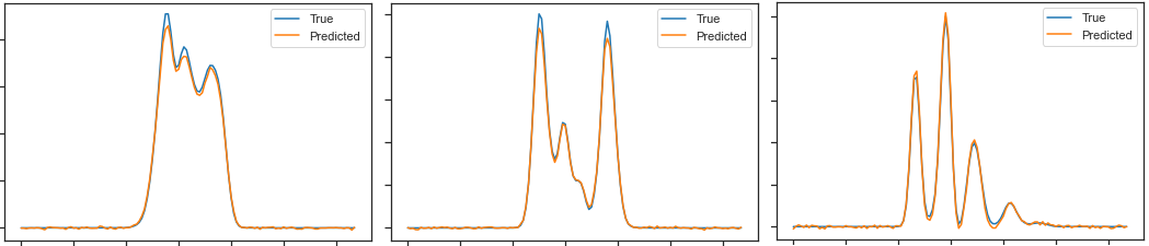
Then I plot comparative graphs comparing predicted outputs_test with ground-truth labels_test:
nnn = 3 # to chose a specific sample from the first batch of the test dataset (e.g. 3rd data sample in the batch of 100 samples)

figure, ax1 = plt.subplots()
ax1.plot(labels_test[nnn-1,:], color=u'#1f77b4')
ax1.plot(160*outputs_test[nnn-1,:], color=u'#ff7f0e'')
ax1.legend(['True','Predicted'])
ax1.set_ylim([-40,40])
As you can see, I have to multiply the outputs_test by 160 to make the resulting curve comparable in amplitude with the ground-truth curve. This is the first question, why would it be so?
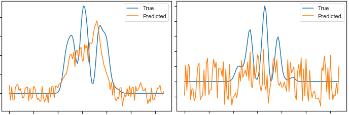
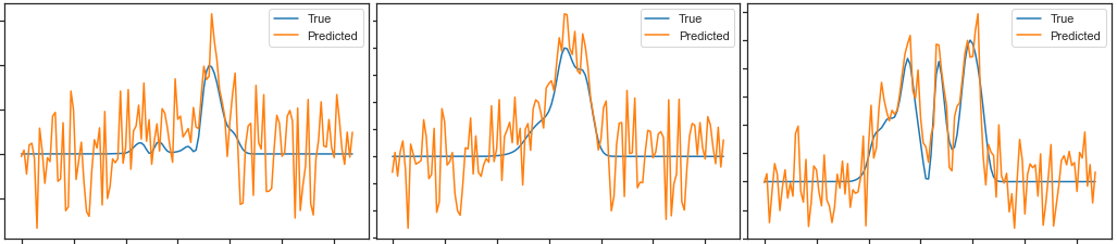
Here are the plots for different data-samples from the batch of 100 and for different epochs of the training (the rows represents indicated epochs and the columns represent indicated data-samples from the batch):
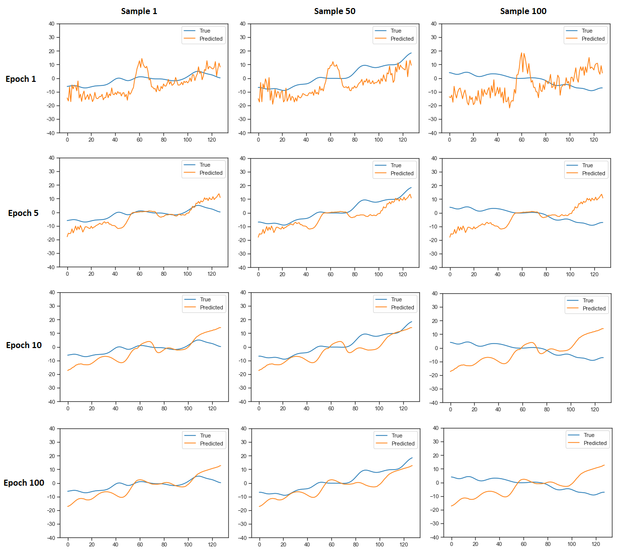
As you can see, the result doesnt depend much on what data-sample is fed into the network. This is another question, why is that so?
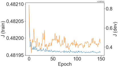
Addon: For the reference this is how cost evolved over 150 epochs.
Also, my network consists of 10 convolutional layers (including batchnorms and maxpools in some places) and 5 linear fully-connected layers.
This is the output of the print(network):
Network(
  (encoder): MyEncoder(
    (conv_blocks): Sequential(
      (0): Sequential(
        (0): Conv2d(1, 6, kernel_size=(5, 5), stride=(1, 1))
        (1): ReLU()
      )
      (1): Sequential(
        (0): Conv2d(6, 12, kernel_size=(5, 5), stride=(1, 1))
        (1): MaxPool2d(kernel_size=2, stride=2, padding=0, dilation=1, ceil_mode=False)
        (2): BatchNorm2d(12, eps=1e-05, momentum=0.1, affine=True, track_running_stats=True)
        (3): ReLU()
      )
      (2): Sequential(
        (0): Conv2d(12, 32, kernel_size=(5, 5), stride=(1, 1))
        (1): ReLU()
      )
      (3): Sequential(
        (0): Conv2d(32, 32, kernel_size=(5, 5), stride=(1, 1))
        (1): ReLU()
      )
      (4): Sequential(
        (0): Conv2d(32, 16, kernel_size=(5, 5), stride=(1, 1))
        (1): MaxPool2d(kernel_size=2, stride=2, padding=0, dilation=1, ceil_mode=False)
        (2): BatchNorm2d(16, eps=1e-05, momentum=0.1, affine=True, track_running_stats=True)
        (3): ReLU()
      )
      (5): Sequential(
        (0): Conv2d(16, 16, kernel_size=(5, 5), stride=(1, 1))
        (1): ReLU()
      )
      (6): Sequential(
        (0): Conv2d(16, 14, kernel_size=(5, 5), stride=(1, 1))
        (1): ReLU()
      )
      (7): Sequential(
        (0): Conv2d(14, 14, kernel_size=(5, 5), stride=(1, 1))
        (1): BatchNorm2d(14, eps=1e-05, momentum=0.1, affine=True, track_running_stats=True)
        (2): ReLU()
      )
      (8): Sequential(
        (0): Conv2d(14, 12, kernel_size=(5, 5), stride=(1, 1))
        (1): ReLU()
      )
      (9): Sequential(
        (0): Conv2d(12, 12, kernel_size=(5, 5), stride=(1, 1))
        (1): MaxPool2d(kernel_size=2, stride=2, padding=0, dilation=1, ceil_mode=False)
        (2): BatchNorm2d(12, eps=1e-05, momentum=0.1, affine=True, track_running_stats=True)
        (3): ReLU()
      )
    )
  )
  (decoder): MyDecoder(
    (fc_blocks): Sequential(
      (0): Sequential(
        (0): Linear(in_features=48, out_features=120, bias=True)
        (1): ReLU()
      )
      (1): Sequential(
        (0): Linear(in_features=120, out_features=60, bias=True)
        (1): ReLU()
      )
      (2): Sequential(
        (0): Linear(in_features=60, out_features=40, bias=True)
        (1): BatchNorm1d(40, eps=1e-05, momentum=0.1, affine=True, track_running_stats=True)
        (2): ReLU()
      )
      (3): Sequential(
        (0): Linear(in_features=40, out_features=20, bias=True)
        (1): ReLU()
      )
      (4): Sequential(
        (0): Linear(in_features=20, out_features=10, bias=True)
        (1): ReLU()
      )
    )
  )
  (last): Linear(in_features=10, out_features=128, bias=True)
)