Sigmoid and BCELoss

[snip3r77]

Hi @KFrank
thanks for your prompt reply

I think I got it already

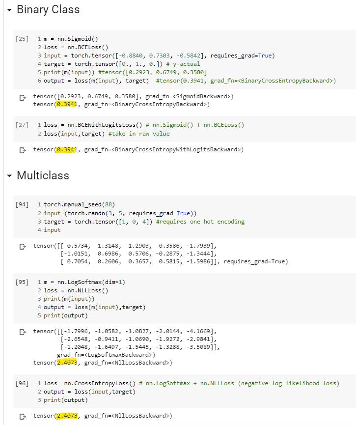
But I have some confusion for crossentropy.

I kinda understand regarding the dim=1 which came from the screenshot below.

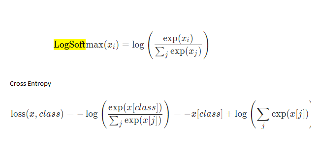
We need to sum up the denominator for both but why we do not require dim for CrossEntropyLoss

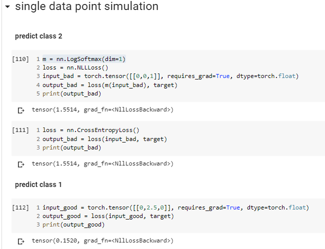
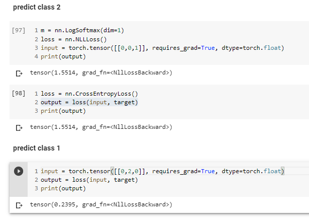
Is my understanding correct when I try so simulate a bad prediction and a good one?
For the target(y_actual),we need to do one hot encoding too.

Also, how can we simulate the NLL?

Understanding NLLLoss function

m = nn.LogSoftmax(dim=1) loss = nn.NLLLoss() # input is of size N x C = 1 x 3 input = torch.tensor([[0,0,0]], requires_grad=True, dtype=torch.float) # each element in target has to have 0 <= value < C target = torch.tensor([1]) output = loss(m(input), target) print(output) _Output: tensor(1.0986, grad_fn=<NllLossBackward>)_ I read the Documentation but it’s not clear. Can someone explain the math behind this example?

we need to exp and then multiply by -1

Sidetrack, in DL if we’re saying logits does it mean raw form as in our input in the codes?
after we apply sigmoid or softmax, it will be probability?

Thanks.