Adding non derivable Wasserstein from scipy to pytorch MSE Works?

[Aymen_Tlili]

Hi i’m trying to use Optimal transport’s Wasserstein distance in pytorch.Before I had known about Geomloss (Getting started — GeomLoss) and their pytorch implementation of an approximation of it , I tried using the exact wasserstein distance on each predicted vector in a batch . “output[0]” represents the predicted batched and “tg” being the target being approximated .

reading Adding a float variable as an additional loss term works? I understand that adding constants(in that batch) gives a gradient of 0 so it should not affect back propogation whatsover but for me it does!
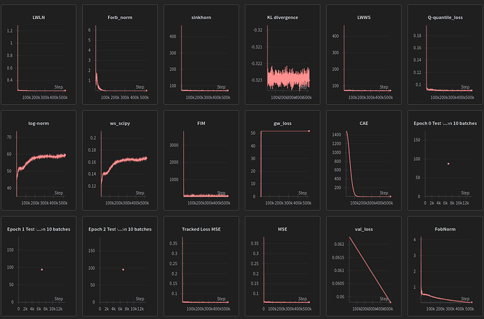
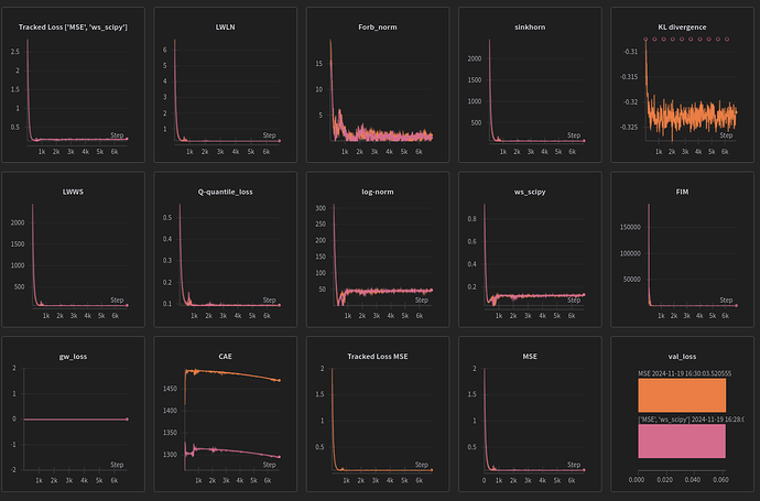
A model trained to do regression with MSE alone is being out performed MSE+Scipy’s WS implementation , in fact this combination is even better than the sinkhorn approximation+MSE combo by a notable margin later down the road .

MSE+ws_scipy can be used in loss.backward() and accelerator.backward(loss) but if u use ws_scipy alone things break because there is no graph behind it telling where to send the gradients to .pure MSE obviously doesn’t have this limitation.

My explination on this is that scipy’s term doesn’t create gradients but it’s presence increases MSE norm and that even in small variation(it’s own gradients alone couple with a big norm) is propagating WS information when it shouldn’t

an analogy is that I imagine the losses being partners .Each has a gradient (money) and a graph of norms(describing where to invest that money at) . Somehow in this combination WS has no money(not derivable by pytorch) and should therefore have no say in things but by injecting it’s norm in MSE’s graph it’s implifying MSE decision by increasing the norm sent through MSE’s graph alone .

if for neurone #250 it’s decided MSE small error , WS big error . WS shouldn’t affect the learning of it and should fall flat on it’s own but it’s somehow affecting MSE’s decision and sending big error still

here is code that shouldn’t work but does and outperforms MSE criterion alone

@ptrblck my hero in shining armor show me the way of the graphs (that we shouldn’t detach)

            vec1_np = output[0].detach().cpu().numpy()
            vec2_np = tg.detach().cpu().numpy()
            # Compute Wasserstein distance for each pair of vectors
            wsd_list = [wasserstein_distance(vec1_np[i], vec2_np[i]) for i in range(vec1_np.shape[0])]
            # If you need an aggregate measure, you can compute the average distance
            average_wsd = sum(wsd_list) / len(wsd_list)
            loss_tr = criterion(output[0],tg)+average_wsd
         accelerator.backward(loss_tr)

[figure of MSE alone being the training metric and logging ws_scipy metric increasing despite sinkhorn’s decreasing ]

[figure of MSE+ws_scipy being significantly different despite running on the same seed]

seed=74
torch.manual_seed(seed)
np.random.seed(seed)
random.seed(seed)

here’s my github for this GitHub - AymenTlili131/Federated-Continual-learning-: PFE
Any help is appreciated before I crack open both libraries and start comparing implementations, I’d like to hear the opinions of people who contributed to them

scipy==1.12.0
torch==1.12.1+cu113 (on RTX 3060 ubuntu22)
torch_geometric==2.4.0
torchaudio==0.12.1
torchdata==0.5.1
torcheval==0.0.7
accelerate==0.30.1

[KFrank]

Hi Aymen!

@Aymen_Tlili

I understand that adding constants(in that batch) gives a gradient of 0 so it should not affect back propogation whatsover but for me it does!

This is unlikely to be true (so it is likely that there is something else going on).

It is hypothetically possible that adding a value that is not part of the
computation graph could affect backpropagation and training. This could
occur due to finite floating-point precision.

Edit: I’ve changed my mind about this. Adding a constant (with requires_grad = False)
to a loss value can introduce round-off error to the result of that addition, but I can’t
think of a way that doing so can pollute, or otherwise change, gradients obtained by
backpropagating that result. Here is a simple illustration:

>>> import torch
>>> torch.__version__
'2.5.1'
>>> p = torch.tensor ([1.0], requires_grad = True)
>>> (2 * p + 3).backward()
>>> p.grad
tensor([2.])
>>> p.grad = None
>>> (2 * p + float ('inf')).backward()
>>> p.grad
tensor([2.])
>>> p.grad = None
>>> (2 * p + float ('nan')).backward()
>>> p.grad
tensor([2.])

For example, if your scipy result, average_wsd, were several of orders of
magnitude larger than the differential piece, criterion(output[0],tg),
the gradient of the differentiable piece could be degraded by round-off error
due to having been added to a much larger value. If you only see a discrepancy
after many training iterations, it could be that very small differences from a single
pass accumulate and get “amplified” as several rounds of training progress.

Is there any way you could post a super-small, fully-self-contained, runnable
example script that reproduces this behavior? Ideally, could you capture the
suspicious behavior by seeing differences in the gradients (.grad of various
parameters) after a single backward pass?

Your reasoning that adding a term to the loss function that is not part of the
computation graph will not mathematically affect backpropagation is correct
(although it could affect things numerically).

Best.

K. Frank

[Aymen_Tlili]

Hey Frank ,
thanks for the input and for reminding me of my netiquette to give a small reproducible example like this : Google Colab if sharing works if not here is class declarations :

import torch
from torch.utils.data import Dataset, DataLoader
import torch.nn as nn
import torch.optim as optim
import numpy as np
import random
import copy

seed=74
torch.manual_seed(seed)
np.random.seed(seed)
random.seed(seed)


# Create a PyTorch-ready dataset
class ToyRegressionDataset(Dataset):
    def __init__(self, n_samples=10000, noise=0.1):
        # Generate random input data (features)
        self.x = torch.linspace(-10, 10, n_samples).unsqueeze(1)  # Shape: (n_samples, 1)
        # Generate labels (targets) based on the quadratic equation with noise
        self.y = 3 * self.x**2 + 2 * self.x + 1 + noise * torch.randn_like(self.x)
    
    def __len__(self):
        return len(self.x)
    
    def __getitem__(self, index):
        return self.x[index], self.y[index]

# Instantiate the dataset and dataloader
dataset = ToyRegressionDataset()
dataloader = DataLoader(dataset, batch_size=25, shuffle=True)

# Define a simple regression model
class RegressionModel(nn.Module):
    def __init__(self):
        super(RegressionModel, self).__init__()
        self.model = nn.Sequential(
            nn.Linear(1, 64),
            nn.ReLU(),
            nn.Linear(64, 32),
            nn.ReLU(),
            nn.Linear(32, 1)
        )
    
    def forward(self, x):
        return self.model(x)

and the cell that mixes it all (MSE + regularizing ws to scame scale as MSE X ws)

# Initialize the model, loss function, and optimizer
model_ws_reg=copy.deepcopy(model1)
criterion = nn.MSELoss()
optimizer = optim.Adam(model_ws_reg.parameters(), lr=0.01)

# Training loop
n_epochs = 1001
for epoch in range(n_epochs):
    b_i=0
    for x_batch, y_batch in dataloader:
        # Forward pass
        predictions = model_ws_reg(x_batch)
        loss = criterion(predictions, y_batch)
        vec1_np = predictions.detach().cpu().numpy()
        vec2_np = y_batch.detach().cpu().numpy()

        wsd_list = [wasserstein_distance(vec1_np[i], vec2_np[i]) for i in range(vec1_np.shape[0])]
        # If you need an aggregate measure, you can compute the average distance
        average_wsd = sum(wsd_list) / len(wsd_list)
        loss = criterion(predictions,y_batch)+average_wsd*0.0001
        # Backward pass and optimization
        if b_i==0 and epoch==0 :
          for name, param in model_ws_reg.named_parameters():
            if param.grad is not None:
                print(f"Parameter: {name} {param}, Gradient: {param.grad[:10]}")
                break
        optimizer.zero_grad()
        loss.backward()
        optimizer.step()
        if b_i==0 and epoch==0 :
          for name, param in model_ws_reg.named_parameters():
            if param.grad is not None:
                print(f"Parameter: {name} {param}, Gradient: {param.grad[:10]}")
                break
        b_i=b_i+1
    if (epoch) % 50 == 0:
        print(f"Epoch [{epoch+1}/{n_epochs}], Loss: {loss.item():.4f}")
for name, param in model.named_parameters():
  if param.grad is not None:
    print(f"Parameter: {name} {param}, Gradient: {param.grad[:10]}")
    break
# Test the model on new data
x_test = torch.linspace(-10, 10, 10000).unsqueeze(1)
y_test = 3 * x_test**2 + 2 * x_test + 1
y_pred = model_ws_reg(x_test).detach()

# Plot the results
import matplotlib.pyplot as plt

plt.figure(figsize=(8, 6))
plt.scatter(dataset.x, dataset.y, label="Original Data", color="blue", alpha=0.5)
plt.plot(x_test, y_test, label="True Function", color="green")
plt.plot(x_test, y_pred, label="Model Prediction", color="red")
plt.legend()
plt.title("Regression Model Fit")
plt.show()

The print outputs are as follows (from left to right : MSE , MSE+ws_scipy , MSE+0.0001ws_scipy )
for 1000 data points and a batch size of 2 intended to create many training steps the results are identical and 100 epochs .

in the example i’m running now i’ve tried to increase those by 10s or 100 folds but even with that and for context key dissimalirities between this and my first post . my first post is working on batchs of 25 1d vectors of lengths 2464 . there’s approximately 13500 examples of these 1D vectors in the trainset and the model is a double input transformer subject to gradient clipping and differing learning rates for each part of it .

and learning rates

the toy example is trying to fit this curve but I don’t know if the scale of values is comparable but i understand your motivation to showcase the change happening after one step , which there is none of here

Hope the info helps and gives more context

update after the increases 100folds : the code I’m posting here is about 1000 epochs instead and here is the same comparison left to right . I’m assuming tracking the first named neurone is enough as params are put in an ordered dict data structure to my knowledge,correct me if not.
(note also i didn’t enforce my package versions to deny that this problem stems from a certain old interaction that might’ve already been debugged)

so the end model is the same but u can notice at the start of training that the gradients were different . I think the fact that the toy example is simple led to this unique solution .Arguably for a much complex task that gradient should cause differing end results if caught before convergence (i.e 900 epochs for a giga transformer)

now the tragic part about this is that the lack of regularization and the WS oversaturating the numerical result is causing better results for my original experiment

[KFrank]

Hi Aymen!

@Aymen_Tlili

a small reproducible example like this :

That’s too much for me to wade through.

Your claim is that adding a scipy result – so not part of the computation graph – to
your loss function changes the result of backpropagation. If this claim is true, you
should be able to demonstrate it with a single forward and backward pass. So you
shouldn’t need many (or any) epochs of training to see it.

Can you reproduce this with something truly minimal? (No DataLoader, no optim,
etc., just a single forward and backward pass with a super-simple toy model and
hard-coded example data.)

Use a divide-and-conquer strategy to “capture” where the effect first shows up and
the data that causes it. Then post just the relevant code in a trimmed-down script
together with the results you get when you run it.

Also, please don’t post screenshots of textual data. Doing so breaks accessibility,
searchability, and copy-paste.

Note, I no longer think that round-off error could be a possible explanation for what
you’re seeing. See the edit to my previous post.

Best.

K. Frank

[Aymen_Tlili]

Hey again Frank Thanks for the feedback and keeping the best for everyone in mind .

I got rid of optimizers and dataloaders and just created fixed tensors to work x and y
note I tried to use a batch size of 25 for both experiments but for one I tried 100 elements in the second dimension and in the second I increased that number of columns to 2464 .

The first step seems to be in all ways i can measure identical between the 2 distances in large and small column numberscenarios so I increased the number of iteration after confirming on 1 step

What i noticed when training this singular neurone is that for 100 columns torch.rand(25, 100) the results were identical even after 10 million iterations when comparing mse to mse+ws_scipy

And for the second experiment running this code on torch rands torch.rand(25, 2464) the results are identical.

So the effect does not appear at this scale for a single neurone or even after a single pass .
I’ll try to up things a notch and use a dense layer and bit by bit reproduce the toy example proved the phenomenon in my last response .

# Set seed for reproducibility
torch.manual_seed(42)
# Sample toy dataset
x = torch.rand(25, 2464)# Input features
y = torch.rand(25, 2464)# Ground truth (targets)
# Initialize parameters
w = torch.tensor(0.5, requires_grad=True)  # Weight
b = torch.tensor(0.5, requires_grad=True)  # Bias
learning_rate = 0.0001
for iteration in range(1000):
  y_pred = w * x + b
  vec1_np = y_pred.detach().cpu().numpy()
  vec2_np = y.detach().cpu().numpy()
  wsd_list = [wasserstein_distance(vec1_np[i], vec2_np[i]) for i in range(vec1_np.shape[0])]
  
  average_wsd = sum(wsd_list) / len(wsd_list)

  loss = torch.mean((y_pred - y) ** 2)#+average_wsd
  if iteration%100==0:
    print(iteration , "Before loss backward \t",w.grad , b.grad)
  loss.backward()
  if iteration%100==0:
    print(iteration , "After loss backward \t",w.grad , b.grad ,"\t Loss \t", average_wsd , loss)
  with torch.no_grad():
      w -= learning_rate * w.grad
      b -= learning_rate * b.grad
  w.grad.zero_()
  b.grad.zero_()
  if iteration%100==0:
    print(iteration,"After with torch no_grad \t",w.grad , b.grad)

the results for a single forward backward pass’s and many more after are the gradients (first 2 numbers one for weight and one for bias)

with ws_scipy

0 Before loss backward 	 None None
0 After loss backward 	 tensor(0.3343) tensor(0.4997) 	 Loss 	 0.2498602782064058 tensor(0.4166, grad_fn=<AddBackward0>)
0 After with torch no_grad 	 tensor(0.) tensor(0.)
1000 Before loss backward 	 tensor(0.) tensor(0.)
1000 After loss backward 	 tensor(0.2703) tensor(0.3819) 	 Loss 	 0.20119250731857183 tensor(0.3395, grad_fn=<AddBackward0>)
1000 After with torch no_grad 	 tensor(0.) tensor(0.)
.
.
.
9000 Before loss backward 	 tensor(0.) tensor(0.)
9000 After loss backward 	 tensor(0.0746) tensor(0.0292) 	 Loss 	 0.1610148009207922 tensor(0.2552, grad_fn=<AddBackward0>)
9000 After with torch no_grad 	 tensor(0.) tensor(0.)

without

0 Before loss backward 	 None None
0 After loss backward 	 tensor(0.3343) tensor(0.4997) 	 Loss 	 0.2498602782064058 tensor(0.1667, grad_fn=<MeanBackward0>)
0 After with torch no_grad 	 tensor(0.) tensor(0.)
1000 Before loss backward 	 tensor(0.) tensor(0.)
1000 After loss backward 	 tensor(0.2703) tensor(0.3819) 	 Loss 	 0.20119250731857183 tensor(0.1383, grad_fn=<MeanBackward0>)
1000 After with torch no_grad 	 tensor(0.) tensor(0.)
.
.
9000 Before loss backward 	 tensor(0.) tensor(0.)
9000 After loss backward 	 tensor(0.0746) tensor(0.0292) 	 Loss 	 0.1610148009207922 tensor(0.0942, grad_fn=<MeanBackward0>)
9000 After with torch no_grad 	 tensor(0.) tensor(0.)

the only difference is that the norm of the loss is bigger but from the gradients and identical results we can infer that only the graph having MSE is back propagated .

I’ll upscale things with an optimizer and later a dense layer and follow the divide and conquer method . Thanks , any hypothesis or experiment ideas are welcome as we unravel this
Kind regards