Hello! I have 10000 tuples of numbers (x1,x2,y) generated from the equation: y = np.cos(0.583*x1)+np.exp(0.112*x2). I want to use a NN like approach in pytorch to find the 2 parameters i.e. 0.583 and 0.112 using SGD. Here is my code:
class NN_test(nn.Module):
    def __init__(self):
        super().__init__()
        self.a = torch.nn.Parameter(torch.tensor(0.7))
        self.b = torch.nn.Parameter(torch.tensor(0.02))

    def forward(self, x):
        y = torch.cos(self.a*x[:,0])+torch.exp(self.b*x[:,1])
        return y

model = NN_test().cuda()

lrs = 1e-4
optimizer = optim.SGD(model.parameters(), lr = lrs)
loss = nn.MSELoss()

epochs = 30
for epoch in range(epochs):
    model.train()
    for i, dtt in enumerate(my_dataloader):
        optimizer.zero_grad()

        inp = dtt[0].float().cuda()
        output = dtt[1].float().cuda()

        ls = loss(model(inp),output)

        ls.backward()
        optimizer.step()
    if epoch%1==0:
        print("Epoch: " + str(epoch), "Loss Training: " + str(ls.data.cpu().numpy()))
where x contains the 2 numbers x1 and x2. In theory it should work easily, but the loss doesn’t go down. What am I doing wrong? Thank you!
I think you are trying to solve a problem that is hard to solve with
gradient descent.
I don’t see any obvious errors in your code. (I looked at it briefly,
but not in detail.) So I don’t think that you’re doing anything “wrong.”
Because you add your x1 and x2 terms together, your problem
decouples into to solving for the two parameters independently.
So let us look at just the cos() piece.
The oscillatory nature of cos() means that your loss function will
likely have several local minima in which the gradient-descent
minimization algorithm can get “stuck.” Whether this happens will
depend on the range and distribution of the x1 you use (which you
didn’t tell us).
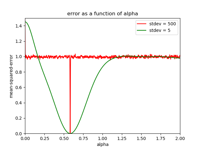
To illustrate this I run two examples: First I sample 10,000 values of x from a gaussian distribution with a mean of zero and a standard
deviation of 5.0, and then again with a standard deviation of 500.0,
and calculate y = np.cos (0.583 * x).
I then try to fit 0.583 with trial values of alpha running from 0.0 to 2.0
by calculating y_alpha = np.cos (alpha * x), and calculating the
mean-squared-error of the y_alpha with respect to the “ground-truth” y.
Here is a plot of the mean-squared-error vs alpha for both values
of the standard deviation:
As you can see in both cases the loss function takes on a global
minimum of 0.0 for alpha = 0.583. So far, so good. But for
stdev = 500, the global minimum is hiding in a tiny range of alpha
surrounded by lots of shallow local minima. Unless you get lucky
and start very close to 0.583 (and for stdev = 500, your starting
value of 0.7 is not close), nothing about your gradient will tell you
that a deep global minimum exists, and your gradient-descent
algorithm won’t converge to the global minimum.
On the other hand (for the ensemble of values of x that I’ve generated
for this example) for stdev = 5, your starting value of 0.7 is well within
the basin of the global minimum, and gradient descent should converge
nicely to the global minimum (for adequately small values of the learning
rate). However, if you were to start out above about 1.25 (or jump up
above 1.25 because of an overly-large learning rate), you could get
stuck in the local minimum around alpha = 1.5) (or one of the local
minima that occur for still larger values of alpha).
(The batch size you use in your training loop – which you didn’t tell
us – will also affect how “noisy” your loss.backward() gradients
are and how much your optimizer jumps around, but this doesn’t
change the essence of what is going on.)
Note, exp() doesn’t have the oscillatory behavior that is the root
cause of the local minima.
So try doing a one-dimensional problem where you just have exp (0.112 * x), and when you get that working, try a
two-dimensional problem where you replace cos() with exp(),
i.e., y = exp (0.583 * x1) + exp (0.112 * x2). That should
be an “easy” minimization problem, so please follow up with further
questions if you can’t get that to work.
Thank you a lot for your reply! I understand what you mean, however I am still a bit confused. Shouldn’t gradient descent take care of this (my batch size was 512), and make sure I reach the global minima after a few iterations? Mainly, my confusion is this: in a normal NN (say for image recognition) one is able to fit a very complex and highly non linear function with (say) 64x64 inputs and several outputs, millions of parameters, a lot of local minima and without much effort (and less training examples) and get very good parameters. In my case, the function is a lot simpler, already written in the desired mathematical form and having just 2 parameters and yet the parameters are sometimes even double than their desired value. I am not sure I understand why does it perform so badly here, compared to a significantly more complex NN.
I also tried using np.sqrt(0.583x1)+np.exp(0.112x2) instead, so no oscillations, and still not getting convergence, using the ranges:
I implemented this from scratch based on your description and provided partial code samples and it works for me: the loss value decreases steadily over time. Hope it helps:
No. In general gradient descent will drive you to the nearest local
minimum, after which you will stay there. (Putting in big jumps by
hand, using large step sizes (large learning rate), or the randomness
from using a batch (instead of averaging the gradient over the whole
training set) can – but won’t necessarily – take you out of a local
minimum.)
Let me give you two bits of intuition. These things might not be true,
but it’s how I think about it.
First, when you train a neural network, you aren’t trying to find the
one, true (with respect to the training set) global minimum. You’re
looking for one of potentially many similar good / good enough / very
good local minima. (In fact, in many real-world cases, if you try to
drive your model parameters to “too good” a minimum (global or not)
you encounter over-fitting where your performance on an out-of-sample
test set starts getting worse, even as your performance on you training
set keeps getting better.)
Second, in higher-dimensional parameter spaces there is “more
room” (more directions) to move around, so you can escape from
what would have been a local minimum in a lower-dimensional
parameter space by moving “around” the barrier that would have
kept you in the local minimum by moving in one of the other directions.
(Having made such a bold assertion, I must confess that I find it very
hard to develop intuition about the structure of the loss-function surface
in these very-high-dimensional parameter spaces.)
That should work fine. Take a look at the code that Katherine posted,
and see why hers works and yours doesn’t.
If you can’t get your version working, feel free to post a complete,
runnable script (preferably one-dimensional, just to make things
simpler) that illustrates the problems you are still having.
x1 will range over [0, 10) and the argument of cos() in x1’s
contribution to y will range over [0, 5.83). That is less than one
full period of cos() ([0, 2 * pi = 6.28)), so you won’t see multiple
oscillations, you won’t see a forest of local minima, and your starting
point for a of 0.7 should be well within the basin of attraction of the
global minimum.
(The gaussian distribution that I used for the plot in my earlier post
and your uniform distribution are not fully comparable, but the standard
deviation of your uniform [0, 10) distribution is 2.89, not too different
from my standard deviation of 5, so the scale of the global minimum’s
basin will be broadly similar in the two cases.)