It appears that the most common task that CNN models perform is classification. Given enough training data, CNNs excel at taking an unknown data item (e.g. an image) and assigning it to one of a set of predefined categories.
I’m looking for pointers, suggestions or guidance for moving beyond classification to a more generalized response based on image features. Specifically, I have images of gravel with a mix of particle sizes. My output is a 5 element vector of values that represent the relative proportion of particles in different size categories. My goal is to use ML to “measure” the proportions of different sizes in unknown images.
I’ve trained a fairly simple CNN (4 conv layers, 3 fully connected) to a quite high level of accuracy - if the input image more or less matches one of the particle size distributions in the training data set. However, if I test an image with a different distribution than any the network has seen during training, the results are typically poor. That is, the results are neither an accurate representation of the true particle distribution (which is what is really desired) nor the closest match from among the distributions that the network has seen during training.
It seems that what my model has learned is basically a classification with a five-element label.
Can anyone suggest a way to proceed? With data augmentation, I currently have about 22,000 input images, in 25 different distribution groups. I am considering adding more images, from additional, different distributions, but acquiring this data will be time-consuming. Do you think it’s likely to improve the performance?
I’ve considered transfer learning. For instance, some papers have claimed that ResNet learns many texture features (which I believe is likely the main type of information needed for my task). However, ResNet was designed for classification. Can I somehow adapt it to my more general objectives?
I am a relative newcomer to machine learning, so I apologize in advance if the answer to this question is obvious.
May I ask some clarifying questions about your use case?
Leaving aside your current network and the kind of annotations you
have for your data, ideally, what would you like the output of your
network to be? Would you like the full probability distribution of
particle sizes – that is, roughly speaking, a histogram of particle sizes
with lots of bins?
Is it important that you use neural networks / machine learning for this
task, or would you be open to using other computer-vision techniques?
What, in more detail, is the meaning of these five numbers? Are your
ground-truth annotations analogous length-5 vectors that have the
same meaning?
What loss function are you using to compare your network outputs
to your annotations?
What does the final layer of your network look like – that is what is
the layer that produces this length-5 output?
Are the test images that your network does poorly on in any way
different in character than the images you used to train your network,
or are they basically the same? For example, did you randomly
select some test images from the same larger annotated set from
which you selected your training set?
In general, if you are getting significantly worse results on test images
that are of the same character as you training images, you are seeing
signs of overfitting. That is, your network has been trained enough
times on the same images that in addition to “learning” the properties
you want it to learn, it is also learning recognize individual images
by their individual peculiarities. Having recognized a specific image,
the network now “parrots back” the “right” answer.
The “rigorous” approach is to split your annotated data set into three
pieces (usually randomly) – a training set, a validation set, and a test set. You use your training set to train with backpropagation and
optimizer parameter updates. At times of your choosing (for example,
once every epoch), you calculate your loss and potentially other
evaluation metrics for your validation set, and use this information to
decide when to stop, perhaps because the results are good enough,
or training has slowed down, or overfitting has set in.
Only after you have settled on your “final” trained network, do you
apply it to your test set to see how well it actually performs. (The
purist notion of rigor here is that using your validation set to evaluate
the performance of your final network would constitute a “data leak”
because you did use the validation set as part of your training process.)
How many unaugmented annotated images do you have? How big
are the images, and are different regions of a given images relatively
independent so that it might be reasonable to consider different regions
of a single image as independent data samples?
What is a “distribution group?” What is the relationship of a distribution
group and the 5-element output of your network?
Related to the question of whether your ground-truth annotations have
the same structure as your network output, what is the relationship of
a distribution group to your annotations?
My gut feeling is that ResNet is unlikely to be helpful for you (but I
could well be wrong).
My intuition – not based on any real experience or evidence – about
transfer learning goes something like this:
The upstream layers of something like ResNet “learn” low-level
“features” – things like edges and arcs and maybe blobs. In the
middle these get aggregated together into mid-level features like
nose-like blobs and eye-like blobs. In the final, down-stream layers
they get aggregated into faces, cat-like faces, dog-like faces, and
ultimately, into cat-vs-dog predictions.
As you say, upstream ResNet layers recognize “textures” so it’s
plausible that pre-trained, upstream ResNet layers could be a useful
starting point for your training. But your ultimate task (as I understand
it) is really quite different than what ResNet was trained for, so I’m not
convinced that you would get that much benefit using it as a starting
point.
Leaving aside your current network and the kind of annotations you
have for your data, ideally, what would you like the output of your
network to be? Would you like the full probability distribution of
particle sizes – that is, roughly speaking, a histogram of particle sizes
with lots of bins?
Five bins is standard for this application. But yes, I’m basically looking for a histogram, aggregated to these five bins and normalized so the total of all bins is 1.0.
Is it important that you use neural networks / machine learning for this
task, or would you be open to using other computer-vision techniques?
We’ve actually tried some analytical machine vision to identify individual particles. Results were quite poor. I am hoping ML can do better.
What, in more detail, is the meaning of these five numbers? Are your
ground-truth annotations analogous length-5 vectors that have the
same meaning?
Yes, ground truth labels mean the same thing. These images were manually acquired from lab samples prepared to have different distributions.
What loss function are you using to compare your network outputs
to your annotations?
RMSE
What does the final layer of your network look like – that is what is
the layer that produces this length-5 output?
nn.linear(32,5), followed by softmax to normalize to 0-1 range.
Are the test images that your network does poorly on in any way
different in character than the images you used to train your network,
or are they basically the same? For example, did you randomly
select some test images from the same larger annotated set from
which you selected your training set?
I have randomly selected 20% of the images as validation images. These do reasonably well though the average loss is higher than for the training images (as I’d expect). I then tried other images which have the same type of annotation but which are not from the original data set. Our goal is transfer to other images.
In general, if you are getting significantly worse results on test images
that are of the same character as you training images, you are seeing
signs of overfitting. That is, your network has been trained enough
times on the same images that in addition to “learning” the properties
you want it to learn, it is also learning recognize individual images
by their individual peculiarities. Having recognized a specific image,
the network now “parrots back” the “right” answer.
Yes, I have come to that conclusion also. However, I realized that even without the overfitting issue I see no sign of the generalization that I am trying for.
The “rigorous” approach is to split your annotated data set into three
pieces (usually randomly) – a training set, a validation set, and a test set. You use your training set to train with backpropagation and
optimizer parameter updates. At times of your choosing (for example,
once every epoch), you calculate your loss and potentially other
evaluation metrics for your validation set, and use this information to
decide when to stop, perhaps because the results are good enough,
or training has slowed down, or overfitting has set in.
Only after you have settled on your “final” trained network, do you
apply it to your test set to see how well it actually performs. (The
purist notion of rigor here is that using your validation set to evaluate
the performance of your final network would constitute a “data leak”
because you did use the validation set as part of your training process.)
Yes, of course… but I’m in exploration mode at the moment. I’ve actually trained several different networks with variations in input image size and augmentation techniques. The results vary somewhat but the pattern is more or less the same.
How many unaugmented annotated images do you have? How big
are the images, and are different regions of a given images relatively
independent so that it might be reasonable to consider different regions
of a single image as independent data samples?
About 2600 different images. They are about 1500x1500 to start. My latest attempt downsamples them to 224x224 (earlier versions used 64x64 and 128x128).
The entire image area is relevant to the answer, because the particles are not uniformly distributed in the image area. One of my earlier attempts used subsetting for augmentation, but I realized the subsets might in fact reflect a significantly different distribution.
What is a “distribution group?” What is the relationship of a distribution
group and the 5-element output of your network?
As noted above, these images were synthetically created by preparing a gravel sample with a particular distribution of particle sizes, spreading it in a frame, and taking a series of photos. There were 25 different samples prepared, each one with a different distribution of particle sizes. For each distribution, the students took about 1000 images, from different locations. After a few images, they would “disturb” the gravel, moving it around to change the patterns, but not the underlying distribution.
What I mean to convey with the term “distribution group” is a set of images all of which have the same 5-element histogram.
As you say, upstream ResNet layers recognize “textures” so it’s
plausible that pre-trained, upstream ResNet layers could be a useful
starting point for your training. But your ultimate task (as I understand
it) is really quite different than what ResNet was trained for, so I’m not
convinced that you would get that much benefit using it as a starting
point.
That is more or less the conclusion I’ve come to. I’ve been looking for papers about using texture in ML. However, pretty much every one is considering a classification task – rather than a “characterization” or “description” task.
Any suggestions would be welcome! (Including your thoughts about non-ML methods.)
So just to confirm: Regardless of any intermediate steps taken in your
overall workflow (e.g., producing a fine-grained histogram or identifying
each individual gravel particle), your final desired goal is to infer a
five-fixed-bin probability distribution. Correct?
This strikes me as not the best way to go.
Your ground-truth is a (discrete) probability distribution and you wish
to predict a matching probability distribution. Cross-entropy is the
natural loss function for such a task. It is a natural measure of how
much two probability distributions differ, and root-mean-squared-error,
while not unreasonable, just isn’t as natural (and the lore is that it
doesn’t work as well for this kind of use case).
Note that pytorch’s CrossEntropyLoss was designed with classification
in mind where you have an integer class label as your target so it
doesn’t apply to your use case. But cross-entropy makes perfect sense
with a probabilistic target (sometimes called “soft labels”).
You can easily write your own probabilistic cross-entropy, as outlined
in this post:
If you go this route, using Linear (32, 5) as your final layer is the
right thing to do, but you will not want to follow it with a softmax()
layer. (Both pytorch’s CrossEntropyLoss and the probabilistic
version I linked to have, for reasons of numerical stability, softmax()
built into them in the form of log_softmax().) That is, you want your
network to output the logits that correspond to your predicted
probabilities, rather than the probabilities themselves.
I can’t say that changing to a cross-entropy loss will necessarily work
great, but it is the first thing I would try.
Training a network that generalizes to inputs that are not entirely of
same character as the training set is an admirable goal, but is harder,
and not always achievable. Regularization techniques (e.g., weight
decay or dropout) do help reduce overfitting, and can help with
generalization to fundamentally different inputs, but are not a panacea.
I would recommend increasing the diversity of your training set to
more completely represent the character of the real-world images
that you will want to analyze “in the wild.”
(More, and better, and more fully representative data, although
potentially expensive, is usually the best first step towards improving
the practical performance of a network.)
Just to confirm, because your network works reasonably well on your
validation images, this is not an issue of overfitting, per se, but one
of generalization.
This is a reasonable number, but more data might well help. (Again,
the size of your images may help in the sense that different regions
of a given image might be sufficiently independent so as to count,
roughly speaking, as separate data samples.)
How much computing power do you have for this project? Can you
reasonably do a lot of long training runs on large models with large
datasets?
Are you downsampling because of hardware limitations, or are you
able to train with the full 1500x1500 images (or more modestly
downsampled images)? I imagine an image of gravel and could
believe that downsampling to 244x244 would lose lots of relevant
information.
Well, if you’ve already tried non-neural-network “particle analysis” and
it doesn’t work, I don’t have much to offer.
In this vein, however, if a person looks at one of your images, are
the individual grains of gravel readily apparent? Do most pixels in
your images belong to a grain of gravel, or do you have a significant
fraction of “background” pixels (e.g., maybe a piece of paper that
your gravel was spread out on)?
How often in your images is a grain of gravel partially occluded by
another grain?
One approach to “particle analysis” – to identify individual grains of
of gravel – would be to train (or fine tune) a segmentation network.
This could either be semantic segmentation where you label each
pixel as gravel body, vs., for example, gravel boundary and / or
background. Or it could be instance segmentation where the network
further infers that one set of “gravel pixels” belongs instance-A of a
gravel grain, and some other set belongs to instance-B.
The significant disadvantage of segmentation is that your training
images would need to be annotated with pixel-by-pixel labels, a
tedious, and potentially expensive task.
Would it be possible for you to post a representative image from your
training set? If the image is too large, posting a cropped, rather than
a downsampled image would be preferable.
Sorry about the delay in replying. I really appreciate your thoughtful responses.
Loss function - I can understand why you’d recommend cross-entropy loss. I chose RMSE because the end users would like to be able to compare the output “error” from the model with the results from the classical machine vision approach. RMSE intuitively captures the overall deviation between an output distribution and the ideal distribution. Cross-entropy loss would be more difficult from them to interpret.
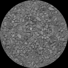
I was startled by your question about downsampling, since I thought this was a standard approach in building CNNs. Wouldn’t a network designed to process 1500x1500 images be enormous? In any case, the particles are quite visible in a 224x224 image (see below). I’m also switching from color to gray scale. Do you think this is a bad idea?
Here’s a downsampled example (downsampled to 224x224 using ImageMagick, not Pytorch transforms):
(The images are normalized before training. This has not been.)
The image area has been cropped to a circle because I am using rotations to do data augmentation.
I think you are right about needing a greater diversity of training data. All these images were taken in the same lab, with the same lighting. I’ll have to discuss this with our end users, to see what they can do.
I recently became aware of some work doing segmentation analysis of this general sort of image using ML, specifically the Mask R-CNN model. Results are excellent, but for training, they had to draw polygons around every single particle in each training image!
My hardware resources are fairly modest, but the ML machine is more or less dedicated to that task, so I can start it up and let it run.
Thank you again for your suggestions. I will update this thread with any progress.
If you have the (hardware/time) bandwidth, it may be a good idea to try training with Cross-entropy loss as the loss function. You may find that this also makes RMSE decrease, possibly even faster than when training with RMSE as the measure of loss.
I agree with G. Philip’s comment. It is perfectly reasonable to use one
loss function for training and one or more distinct loss-like functions
as evaluation metrics. These evaluation metrics might be in some
substantive sense better metrics, or they might be technically not as
good but easier for non-specialists to interpret. Either way, it’s common
practice to use multiple evaluation metrics.
It’s also true, as G. Philip notes, that metric X may improve more
rapidly and end up at a better level if you train with loss A than if
you trained directly with metric X.
In any event, I would strongly recommend that you try training
with cross entropy (or perhaps the Kullback-Leibler divergence,
a related measure of the discrepancy between two probability
distributions). Doing so might not work better than training with
root-mean-squared-error (RMSE), but it certainly could, even
with RMSE as your evaluation metric.
The network, in and of itself, would not be significantly larger, as it
would likely consist of upstream convolutional and downsampling
layers whose sizes are independent of the size of the input images.
However the memory and computation time required to train on
(and evaluate) the large images would be potentially enormous.
The larger particles look distinct to me. In the upper right of your
sample image, around two o’clock, the smaller particles – if that’s
what they are – look to my eye to be harder to distinguish. It’s a
judgement call, but if it’s hard for your eye to see, you would be
making it harder on your network, Perhaps something like 500x500
could provide a happy medium.
My intuition is that gray scale should be fine. Are different particles
of significantly different hues? Are the particles significantly easier
to distinguish by eye in the color image? If not, it doesn’t seem like
a gray-scale conversion would discard much relevant information.
This is perfectly reasonable and possibly helpful. If you do train
with normalization, be sure to evaluate and infer with similarly
normalized inputs.
Indeed!
If you can perform a forward pass and backpropagation on a single
image with your hardware – typically an issue of gpu memory – you
should be able to train, at the cost of hours or days (or even weeks)
of clock / calendar time. (If you can’t run a single sample through
your model, things become much more painful, and it wouldn’t bode
well for managing to carry out training in a reasonable amount of time.)