Bidirectional LSTM isn't 2x the size of 2 Unidirectional LSTMs?

dhruvbird · December 3, 2023, 9:41pm

I expected a bi-lstm to be 2x the size of 2 uni-lstm layers, but a bi-lstm is somehow a bit more than that. Why is that so? i.e. 561k params v/s 2x215k ~= 430k params.

Code:

from torch import nn
from torchinfo import summary

bilstm = nn.LSTM(32, 128, 2, batch_first=True, bidirectional=True)
unilstm = nn.LSTM(32, 128, 2, batch_first=True, bidirectional=False)
print(summary(bilstm))
print(summary(unilstm))

Output:

=================================================================
Layer (type:depth-idx)                   Param #
=================================================================
LSTM                                     561,152
=================================================================
Total params: 561,152
Trainable params: 561,152
Non-trainable params: 0
=================================================================
=================================================================
Layer (type:depth-idx)                   Param #
=================================================================
LSTM                                     215,040
=================================================================
Total params: 215,040
Trainable params: 215,040
Non-trainable params: 0
=================================================================

vdw · December 10, 2023, 7:29am

The problem does not seem to be the number of directions but the number of layers:

from torch import nn

def get_param_count(model):
    return sum(p.numel() for p in model.parameters())

bilstm = nn.LSTM(32, 128, 1, batch_first=True, bidirectional=True)
unilstm = nn.LSTM(32, 128, 1, batch_first=True, bidirectional=False)

print(get_param_count(bilstm))
print(get_param_count(unilstm))

single_layer = nn.LSTM(32, 128, 1)
double_layer = nn.LSTM(32, 128, 2)
triple_layer = nn.LSTM(32, 128, 3)

print(get_param_count(single_layer))
print(get_param_count(double_layer))
print(get_param_count(triple_layer))

If both bilstm and unilstm have the same number of layers, then number of parameters is indeed twice for bilstm. However, if you keep the directionality fixed by double/triple the number of layers, the number of parameters does not double/triple but increases faster.

Sorry, I cannot tell for sure why this is.

J_Johnson · December 11, 2023, 12:50pm

This is more generally the case with any RNN that uses bi-directionality.

We can see what is occurring by printing out the parameters per weight tensor, as follows:

import torch.nn as nn

model = nn.LSTM(20, 50, 3, bias=False)
model2 = nn.LSTM(20, 50, 3, bias=False, bidirectional=True)

for param in model.parameters():
    print(param.size())
print("-----")
for param in model2.parameters():
    print(param.size())

That should produce:

torch.Size([200, 20])
torch.Size([200, 50])
torch.Size([200, 50])
torch.Size([200, 50])
torch.Size([200, 50])
torch.Size([200, 50])
-----
torch.Size([200, 20])
torch.Size([200, 50])
torch.Size([200, 20])
torch.Size([200, 50])
torch.Size([200, 100])
torch.Size([200, 50])
torch.Size([200, 100])
torch.Size([200, 50])
torch.Size([200, 100])
torch.Size([200, 50])
torch.Size([200, 100])
torch.Size([200, 50])

We can then look at the original RNN Bidirectional paper:

A standard RNN layer looks like this:

With each arrow, we have a set of weights. Normally, in an RNN, the above sizes would only differ in that the dim 0 would be the same as the hidden dim, i.e. (50, 20), (50, 50), etc.

The 1 dim of the tensors conveys the input size into that tensor(it may seem counterintuitive to put the output size as dim 0 and input size as dim 1, but this is done for functionality and speed because of how the matmul operation works, not for our viewing convenience, but I digress).

LSTMs have 4x the size of outputs due to the gating channels involved(i.e. 200 for LSTM vs. 50 for RNN in this example), but we’re not delving into that here. We’ll just use the RNN case, as it applies the same to all types of RNNs(LSTM, GRU, etc.).

So each layer in a unidirectional RNN has the weights giving input into the hidden state. Then an activation function is used to decide whether to keep the old state elementwise or use the new. The second set of weights is used after it goes through the activation. Hence the two weights per layer for a unidirectional RNN.

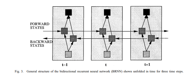
So now we come to the bidirectional RNN:

Drawing from the same paper, we see that there are double the arrows vertically, so 1 layer now has 4 sets of weights instead of 2. Each for forward and backward, two applied to the inputs and two applied to the old state.

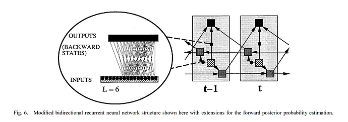
Further in the paper, Schuster proposed a modified BRNN which looks like this:

We can see what gets passed to later layers as inputs are:

The current hidden combined with the last hidden(i.e. torch.cat);
The current hidden combined with the next hidden;

Those yield double the hidden size as an input to the set of weights for subsequent layers.

dhruvbird · December 12, 2023, 5:47am

@J_Johnson I don’t understand where the additional parameters come from.

From: 10.4. Bidirectional Recurrent Neural Networks — Dive into Deep Learning 1.0.3 documentation (which also seems to refer to the same paper)

Fortunately, a simple technique transforms any unidirectional RNN into a bidirectional RNN (Schuster and Paliwal, 1997). We simply implement two unidirectional RNN layers chained together in opposite directions and acting on the same input (Fig. 10.4.1). For the first RNN layer, the first input is �1 and the last input is ��, but for the second RNN layer, the first input is �� and the last input is �1. To produce the output of this bidirectional RNN layer, we simply concatenate together the corresponding outputs of the two underlying unidirectional RNN layers.

it seems like the forward and reverse direction outputs are simply concatenated together (hence no need for additional parameters here). What am I missing?

J_Johnson · December 12, 2023, 12:19pm

The original paper had proposed two BRNNs. The first is what seems to be described in the paper you mentioned. The second, modified BRNN, seems to be what may be implemented in the PyTorch version.

In the diagrams shown above from the original paper, you can also see 2 arrows into the layer output for the original and 3 arrows into the layer output for the modified.

dhruvbird · December 12, 2023, 8:26pm

Got it! This makes sense - i.e. maybe this is the version implemented in PyTorch.

dhruvbird · December 12, 2023, 8:39pm

@J_Johnson I also found this:

The output state is the tensor of all the hidden state from each time step in the RNN(LSTM), and the hidden state returned by the RNN(LSTM) is the last hidden state from the last time step from the input sequence. You could check this by collecting all of the hidden states from each step and comparing that to the output state,(provided you are not using pack_padded_sequence).

And I recall seeing this behaviour myself - i.e. the last output is the final hidden state. If the one in PyTorch is the 2nd BRNN, then the output and hidden states wouldn’t match up eh?

J_Johnson · December 13, 2023, 8:55am

The hidden state will still be the forward and backward hidden states combined. So it should be double the size in the bidirectional case.

And that is the case in the docs. The output size is (L, DxHout), where L is length, D is 1 for unidirectional and 2 for bidirectional, and Hout is hidden out:

https://pytorch.org/docs/stable/generated/torch.nn.LSTM.html

The hidden state is of the same size.