Computation Graph - Higher order gradients with pretrained models

Hello all,

I have the following issue:
I have a function that takes as input a pretrained model (eg. GAN) and another vector y, let’s say
f(y, G(z)) .
I want to compute the gradient of this function w.r.t. to z_i for different (and many) z_i’s. Let us denote this gradient as:

dfdz = []
for i in range(N):
dfdz.append(autorgrad.grad(f(y,G(z_i)),z_i, create_graph= True)[0])

That gradient is a function of y and the jacobian of G(z_i). Then, all the gradients dfdz = [dfdz[1] dfdz[2],…,dfdz[N] ] are given as input to another function g(dfdz,x) and I want to get the gradient of g(dfdz,x) w.r.t. y (let’s denote it as dgdy).

The issue is that when I use create_graph = True, which is needed for being able the gradient of g(dfdz,x), the CUDA memory blows up. I have checked the computation graph and it seems that for each z_i Pytorch saves in memory the computation graph of G(z_i) which is huge.
However, I don’t need the compuation graph for G(z_i) which is a pretrained model. In fact, I only care about its gradients w.r.t. to z (Jacobians).

Is there any way to delete from memory that part of the graph ?
If not, is there any alternative and efficient way to perform the same computations without setting create_graph to True?

Thank you !
You can do the backward in two steps, first compute derivative of f wrt g(z), y, then use the chain rule to compute dfdz. When you do the first stpe, you’d still need create_graph=True because you’d still need to backward through that part of the graph to compute second order wrt y later, but when you compute dfdz, you would be free to pass in create_graph=False.

By chain rule you mean to compute dffz as dffz = dfdG * dGdz ? But dGdz is a jacobian matrix, which is huge…

You don’t need to materialize any jacobian matrix. Consider two functions f, g composed together as g(f(x))

If I do backward in one go, it looks like: dzdx = torch.autograd.grad(z, inputs=x), you can think of this as computing “v^T Jg Jf”. Because we go from left to right, we were dealing with vectors all the way, so we never had to materialize any Jacobian.

If I do backward piece by piece, it looks like: dzdy = torch.autograd.grad(z, inputs=y); dzdx = torch.autograd.grad(y, inputs=x, grad_output=dzdy). You can think of this as computing “u^T = v^T Jg” then doing “u^T Jf”, and it is the same idea as above.

1 Like

Ok, I see why the Jacobian is not materialized and computations can be done efficiently!

Recall now that f(y,G(z)) i.e., f is a function of y and G(z)) where G(z) a pretrained model mapping form n to m with n<<m). What is still not clear to me is the following: Let’s define another scalar function g which takes as input dfdz and another variable x i.e. t = g(dfdz,x). I want to compute the gradient of g w.r.t. y where y implicitly appears in dfdz. How can I compute dgdy given that for the computation of dfdz I have set create_graph = False?? PyTorch can’t see the dependency on y.

If you compute dfdz in two steps: first compute dfdy and dfdG in create_graph=True, then compute dfdz using dfdG and the chain rule in create_graph=False. All the dependency of dfdz on y happens when you do the dfdy and dfdG, so everything is well as long as the that part of the graph was still created, and the rest of the graph shouldn’t matter because whatever is computed there is constant wrt y.

1 Like

I have implemented the two-step apporach you propose but I get

“RuntimeError: One of the differentiated Tensors appears to not have been used in the graph. Set allow_unused=True if this is the desired behavior.”

and even when I set allow_unused=True, it gives None as gradient.

Given the function f(G(z), y), we want to compute the second-order derivative dfdzdy. Naively, we would just use double backward here, but because G is some large pretrained model, we would ideally want to avoid backwarding through that part of the graph. Below, through clever usage of forward AD, we achieve the same result but memory scaling is constant wrt the depth of G.

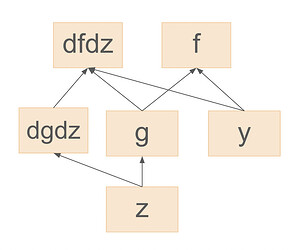
Taking a closer look at the structure of dfdz, the dependency structure of the computed values is as follows (you can kind of think of this as the recorded graph after computing dfdz with create_graph=True):

We observe that because of the chain rule: dfdz is a linear function of dfdg, and dfdg is a function of y and g, i.e., dfdz = A(f(y, g)) where A is some linear function A(v) = v^T Jg.

We also know that because of the chain rule, the gradient of dfdz wrt y can be computed as dfdzdy = grad_out^T J_A J_f, where J_A, J_f are the Jacobian of A and f respectively. Note that in practice, the Jacobians aren’t actually materialized here.

Finally, the key here is to notice that since A is linear, J_A is simply J_g^T, so now we have:

grad_out^T J_g^T J_f = (J_g grad_out)^T J_f

and this is very convenient for us because J_g grad_out is actually the forward grad of g.

In terms of code, this looks like:

import torch
from torch.autograd.forward_ad import dual_level, make_dual, unpack_dual

# Setup
def G(x):
    return x.sum(dim=1).exp()

def f(y, g_out):
    return ((y.sum(dim=1) + g_out) ** 3).sum()

# Using forward AD
z = torch.rand((3, 4))
y = torch.rand((3, 4), requires_grad=True)

with dual_level():
    z_dual = make_dual(z, torch.ones_like(z))
    # Make sure to freeze your model, e.g. set requires_grad=False
    g_out_dual = G(z_dual)
    g_out, g_out_tangent = unpack_dual(g_out_dual)

g_out.requires_grad_(True)
f_out = f(y, g_out)
dfdg_out, dfdy = torch.autograd.grad(f_out, inputs=(g_out, y), create_graph=True)
dfdzdy1, = torch.autograd.grad(dfdg_out, inputs=(y,), grad_outputs=g_out_tangent)

# Compare with the result using double backward
z = z.clone().detach().requires_grad_(True)
y = y.clone().detach().requires_grad_(True)
f_out = f(y, G(z))
dfdz, = torch.autograd.grad(f_out, inputs=(z,), create_graph=True)
dfdzdy2, = torch.autograd.grad(dfdz, inputs=(y,), grad_outputs=torch.ones_like(dfdz))

print(torch.allclose(dfdzdy1, dfdzdy2))  # True
1 Like