Creating a PyTorch model to fit a polynomial distribution

Hello, I am a beginner PyTorch user and have been following some tutorials to learn how to build some very basic PyTorch models. After building a model to fit a linear distribution (01. PyTorch Workflow Fundamentals - Zero to Mastery Learn PyTorch for Deep Learning) I tried to create a model to fit a polynomial distribution.

The code below walks through the data generation, model construction, and training results:

import torch
import numpy as np
from torch import nn
import matplotlib.pyplot as plt

print(f'using version {torch.__version__}')

# create some known parameters
p1 = 2
p2 = -13
p3 = 26
p4 = -7
p5 = -28
p6 = 20
p7 = 1

# generate some data
def poly(x): 
    return p1*x**6 + p2*x**5 + p3*x**4 + p4*x**3 + p5*x**2 + p6*x + p7
size = 100
start = -1
end = 3
X = torch.arange(start, end, (end-start)/size)
y = poly(X) # + torch.normal(0, 0.75, size=(size,)) # if you want to add noise

# Train test split
X_train = torch.cat((X[:40], X[50:]))
y_train = torch.cat((y[:40], y[50:]))
X_test = X[40:50]
y_test = y[40:50]

# Build the model:
class PolynomialRegressionModel(nn.Module):
    def __init__(self):
        super().__init__()
        self.p1 = nn.Parameter(torch.rand( 1,
                                                requires_grad=True,
                                                dtype=torch.float32))
        self.p2 = nn.Parameter(torch.rand( 1,
                                                requires_grad=True,
                                                dtype=torch.float32))
        self.p3 = nn.Parameter(torch.rand( 1,
                                                requires_grad=True,
                                                dtype=torch.float32))
        self.p4 = nn.Parameter(torch.rand( 1,
                                                requires_grad=True,
                                                dtype=torch.float32))
        self.p5 = nn.Parameter(torch.rand( 1,
                                                requires_grad=True, 
                                                dtype=torch.float32))
        self.p6 = nn.Parameter(torch.rand( 1,
                                                requires_grad=True,
                                                dtype=torch.float32))
        self.p7 = nn.Parameter(torch.rand( 1,
                                                requires_grad=True,
                                                dtype=torch.float32))
    def forward(self, x): 
        return self.p1*x**6 + self.p2*x**5 + self.p3*x**4 + self.p4*x**3 + self.p5*x**2 + self.p7*x + self.p7

# Create the model
torch.manual_seed(42)
model = PolynomialRegressionModel()

# Define the loss function and the optimizer
loss_fn = nn.L1Loss()
learning_rate = 0.0001
optimizer = torch.optim.SGD(params = model.parameters(), 
                            lr = learning_rate)

# Train the model
epochs = 10000
epoch_num = []
train_losses = []
test_losses = []
for epoch in range(epochs):
    model.train()
    y_pred = model(X_train)
    loss = loss_fn(y_pred, y_train)
    optimizer.zero_grad()
    loss.backward()
    optimizer.step()

    model.eval()
    with torch.inference_mode():
        test_pred = model(X_test)
        test_loss = loss_fn(test_pred, y_test)

        if epoch % 10 == 0:
            epoch_num.append(epoch)
            train_losses.append(loss.item())
            test_losses.append(test_loss.item())
            print(f'Epoch: {epoch} | MAE train loss: {round(loss.item(), 6)} | MAE test loss: {round(test_loss.item(), 6)}')

using version 1.12.1
Epoch: 0 | MAE train loss: 115.959633 | MAE test loss: 1.532966
Epoch: 10 | MAE train loss: 107.854439 | MAE test loss: 1.515569
Epoch: 20 | MAE train loss: 99.749237 | MAE test loss: 1.503134
Epoch: 30 | MAE train loss: 91.644035 | MAE test loss: 1.497113

Epoch: 3620 | MAE train loss: 3.567217 | MAE test loss: 2.296267
Epoch: 3630 | MAE train loss: 3.564242 | MAE test loss: 2.295868
Epoch: 3640 | MAE train loss: 3.565017 | MAE test loss: 2.296033
Epoch: 3650 | MAE train loss: 3.566075 | MAE test loss: 2.295634

Plot the data:
fig, (ax1, ax2, ax3) = plt.subplots(1, 3, figsize=(15, 5))

# Plot the ground truth
ax1.scatter(X_train, y_train, c='g', label='Training Data')
ax1.scatter(X_test, y_test, c='r', label='Test Data')
ax1.set_xlabel('x')
ax1.set_ylabel('y')
ax1.set_title('y = 2x^6 - 13x^5 + 26x^4 - 7x^3 - 28x^2 + 20x + 1')
ax1.title.set_fontsize(9)
ax1.legend(loc='upper left')

# Plot the training loss
ax2.plot(epoch_num, train_losses, c='b', label='Training Loss')
ax2.plot(epoch_num, test_losses, c='m', label='Test Loss')
ax2.set_xlabel('Epoch')
ax2.set_ylabel('Loss')
ax2.set_title('Training Loss')
ax2.legend(loc='upper right')

# plot the final predictions
ax3.scatter(X_train, y_train, c='g', label='Training Data')
ax3.scatter(X_test, y_test, c='r', label='Test Data')
ax3.scatter(X_train, model(X_train).detach().numpy(), c='b', label='Training Predictions')
ax3.scatter(X_test, model(X_test).detach().numpy(), c='m', label='Test Predictions')
ax3.set_xlabel('x')
ax3.set_ylabel('y')
ax3.set_title('Final Predictions')
ax3.legend(loc='upper left')

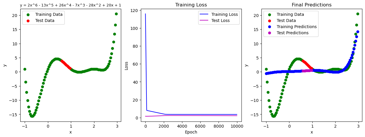
As you can see, the model does a poor job fitting either the training or the test data. I have played around with MSE instead of L1 loss, as well as Adam vs SGD, but no major improvements. I think I’m missing something fundamental in either the model construction or the training loop but I’m not sure what it is.

NOTE: I am sure that there is a fancier built-in approach for fitting this type of distribution. I would be interested in hearing other approaches, but here I am specifically trying to conceptualize what is wrong with this implementation. Any feedback would be greatly appreciated.

Hi Helene!

You have a typo here – you want your linear term to be self.p6*x (not p7).

As such, you are gluing your linear and constant terms together with the
same coefficient, so you can’t expect to fit your original polynomial that well.

Two further comments:

First, this approach to fitting a relatively high-order polynomial is rather
ill-conditioned, so you should expect training to be slow.

Second, because you snip your test data out as a single sub-range of x,
your test data will not be particularly representative of your training data.
If you only look at your test data, you could imagine fitting it well with just
a linear function and quite well with a quadratic. (Your test-data loss is still
a valid measure of how well your model has trained – it’s just a somewhat
incomplete measure because it doesn’t include the values of x where your
polynomial is varying rapidly.)

Best.

K. Frank

Thank you for the quick reply and for pointing out that error! I am still finding that my model can’t fit the distribution, so perhaps it’s time to explore a more appropriate approach.

Hi Helene!

You can fit the polynomial, but training is slow so you might need a
little patience.

Your code will work if you use a lot of epochs. I’m not that patient,
so I added momentum to the SGD optimizer to get the training to
converge more rapidly.

Here is your code, with (minor) modifications noted as comments.

In short, I fixed the self.p6 typo, added momentum to SGD, reduced
the learning rate (for better stability), and increased your number of
epochs by a factor of 100. I also print out the trained values of the
polynomial coefficients at the end

Here is the complete script:

import torch
print (torch.__version__)

_ = torch.manual_seed (2022)


from torch import nn

print(f'using version {torch.__version__}')

# create some known parameters
p1 = 2
p2 = -13
p3 = 26
p4 = -7
p5 = -28
p6 = 20
p7 = 1

# generate some data
def poly(x): 
    return p1*x**6 + p2*x**5 + p3*x**4 + p4*x**3 + p5*x**2 + p6*x + p7
size = 100
start = -1
end = 3
X = torch.arange(start, end, (end-start)/size)
y = poly(X) # + torch.normal(0, 0.75, size=(size,)) # if you want to add noise

# Train test split
X_train = torch.cat((X[:40], X[50:]))
y_train = torch.cat((y[:40], y[50:]))
X_test = X[40:50]
y_test = y[40:50]

# Build the model:
class PolynomialRegressionModel(nn.Module):
    def __init__(self):
        super().__init__()
        self.p1 = nn.Parameter(torch.rand( 1,
                                                requires_grad=True,
                                                dtype=torch.float32))
        self.p2 = nn.Parameter(torch.rand( 1,
                                                requires_grad=True,
                                                dtype=torch.float32))
        self.p3 = nn.Parameter(torch.rand( 1,
                                                requires_grad=True,
                                                dtype=torch.float32))
        self.p4 = nn.Parameter(torch.rand( 1,
                                                requires_grad=True,
                                                dtype=torch.float32))
        self.p5 = nn.Parameter(torch.rand( 1,
                                                requires_grad=True, 
                                                dtype=torch.float32))
        self.p6 = nn.Parameter(torch.rand( 1,
                                                requires_grad=True,
                                                dtype=torch.float32))
        self.p7 = nn.Parameter(torch.rand( 1,
                                                requires_grad=True,
                                                dtype=torch.float32))
    def forward(self, x):
        # replace self.p7*x with self.p6*x
        return self.p1*x**6 + self.p2*x**5 + self.p3*x**4 + self.p4*x**3 + self.p5*x**2 + self.p6*x + self.p7

# Create the model
torch.manual_seed(42)
model = PolynomialRegressionModel()

# Define the loss function and the optimizer
loss_fn = nn.L1Loss()
# learning_rate = 0.0001
learning_rate = 0.00001   # reduce the learning rate for stability
# add momentum to SGD to speed up training dramatically
optimizer = torch.optim.SGD(params = model.parameters(), 
                            lr = learning_rate, momentum = 0.99)

# Train the model
# epochs = 10000
epochs = 1000001   # one hundred times as many epochs
epoch_num = []
train_losses = []
test_losses = []
for epoch in range(epochs):
    model.train()
    y_pred = model(X_train)
    loss = loss_fn(y_pred, y_train)
    optimizer.zero_grad()
    loss.backward()
    optimizer.step()

    model.eval()
    with torch.inference_mode():
        test_pred = model(X_test)
        test_loss = loss_fn(test_pred, y_test)

        # if epoch % 10 == 0:
        if epoch % 100000 == 0:  # print less frequently
            epoch_num.append(epoch)
            train_losses.append(loss.item())
            test_losses.append(test_loss.item())
            print(f'Epoch: {epoch} | MAE train loss: {round(loss.item(), 6)} | MAE test loss: {round(test_loss.item(), 6)}')

# compare fit polynomial coefficients to originals
print ('p1:', p1, model.p1.item())
print ('p2:', p2, model.p2.item())
print ('p3:', p3, model.p3.item())
print ('p4:', p4, model.p4.item())
print ('p5:', p5, model.p5.item())
print ('p6:', p6, model.p6.item())
print ('p7:', p7, model.p7.item())

And here is its output:

1.12.0
using version 1.12.0
Epoch: 0 | MAE train loss: 116.280228 | MAE test loss: 1.51387
Epoch: 100000 | MAE train loss: 2.412973 | MAE test loss: 2.23823
Epoch: 200000 | MAE train loss: 2.027514 | MAE test loss: 1.844248
Epoch: 300000 | MAE train loss: 1.654051 | MAE test loss: 1.46533
Epoch: 400000 | MAE train loss: 1.287786 | MAE test loss: 1.136948
Epoch: 500000 | MAE train loss: 0.917452 | MAE test loss: 0.822819
Epoch: 600000 | MAE train loss: 0.554058 | MAE test loss: 0.49724
Epoch: 700000 | MAE train loss: 0.201879 | MAE test loss: 0.152985
Epoch: 800000 | MAE train loss: 0.664451 | MAE test loss: 0.003946
Epoch: 900000 | MAE train loss: 0.662036 | MAE test loss: 0.003858
Epoch: 1000000 | MAE train loss: 0.661487 | MAE test loss: 0.003569
p1: 2 2.006725311279297
p2: -13 -12.997417449951172
p3: 26 26.000911712646484
p4: -7 -6.99958610534668
p5: -28 -27.99980354309082
p6: 20 20.000106811523438
p7: 1 0.9998350143432617

As a pytorch learning exercise, this is a good task. You might try
using SmoothL1Loss (or, similarly, MSELoss) and see if the Adam
optimizer helps. (It often helps, but can be less stable.) Also play
around with the learning rate and the value for momentum.

I haven’t tried it, but I expect that if you were to package your model
coefficients as a single Parameter of shape [7] and use cumprod()
to compute the powers of x (also as a tensor of shape [7]), you would
probably speed up the forward and backward passes a lot.

(If your real-world use case is to fit polynomials, gradient descent and
pytorch are very much not the right approach.)

Best.

K. Frank

This is the perfect answer, thank you very much for your feedback!