Custom loss function for discontinuous angle calculation

I’m trying to input images of objects that are rotated in the xy plane and use a CNN to learn the angle of rotation in the range 0-360 degrees.

However as mentioned in many posts (eg. Data_Science) , there’s a discontinuity between 0 degrees and 360 degrees where predictions of 359.9 degrees will be penalised heavily when the true value is in fact 0 degrees and so the prediction is very close to the target but the discontinuous nature of the numerical range makes the error huge.

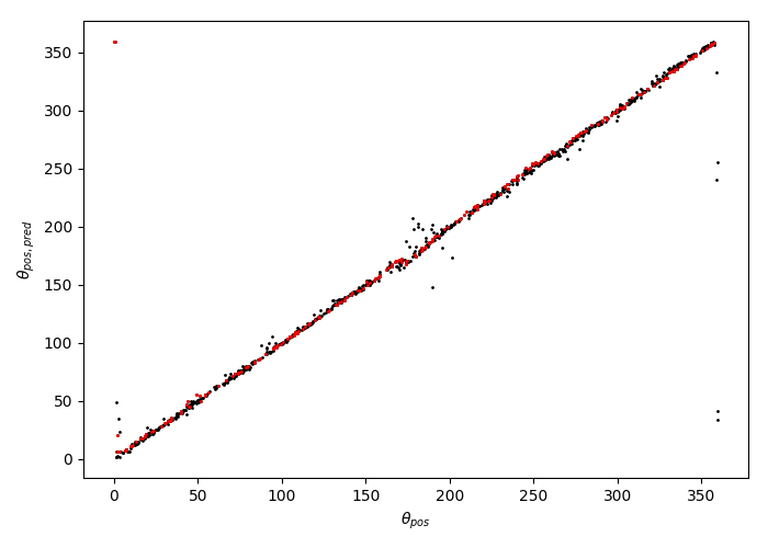
This results in striping at 0 and 360 degrees (and also 180 degrees) - see image below:

I want to write a custom loss function that instead looks to minimise the smallest angle between predicted and true rotation angle given that there are 4 ways in which you can measure the angle between them.

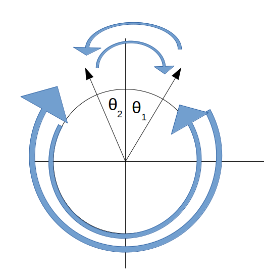
Taking the absolute of these (or the squared angular difference) makes two of these angular measurements equivalent and therefore you only have 2 ways to measure the angular difference between true and predicted angle.

Therefore my custom loss function looks as follows:

def pos_loss(output, target):
   """ LOSS FUNCTION FOR POSITION ANGLE BASED ON MINIMUM ARC SEPARATION """
   loss = torch.mean(torch.stack([ (output-target)**2,
                                  (1-torch.abs(output-target))**2] ).min(dim=0)[0])
   return loss

Note: the 1 in 1-torch.abs(ou... comes from my target being in the range 0-1 as I have normalised the range 0-360 to mean that I can use a sigmoid activation for the output layer and simply get back to the true angle by multiplying up by 360, post training.

And I use the loss function during a CNN training run simply by calling:

loss = pos_loss(prediction,targets)
optim.zero_grad(); loss.backward(); optim.step()

Am I missing a huge step in implementing a custom loss function here that means the way I’m using mine means no appropriate gradients can be calculated?

Using torch.nn.MSELoss() instead trains well but gives striping, but using my custom loss function gives really unstable training that often defaults to predicting close to 0 for all input examples.

Many thanks in advance and please ask as many questions as you’d like.


Extra information:

I am using:
Python 3.6.8
PyTorch 1.0.0

1 Like

Hi :weight_lifting_man:

Your gradients should be fine since you are using pytorch functions. I don’t know about that logic though, looks a bit weird. Try if it gives the same outputs as this function I found on SO.

def angle(angle1, angle2):
    a = angle1 - angle2
    a = (a + 180) % 360 - 180
    print(abs(a))


angle(359, 1)  # -> 2
angle(10, 100)  # -> 90
angle(10, 150)  # -> 140
angle(10, 200)  # -> 170
2 Likes

Apologies for the late reply on this!

I found that your method worked but then your use of quadrants got me thinking about Euler rotation matrices. So I tried instead learning the diagonal components of the rotation matrix and then running an atan2 method of retrieving theta. This worked like a charm in removing the discontinuity at 0/360 degrees and accounts for the quadrants too.

Could you share the loss function? I’m on a same problem here.

I don’t know how in depth you want me to go but here’s some useful info:

I was trying to learn the angle as an output of a network so instead of learning one value I instead learned 2 values corresponding to two components of the rotation matrix about z (R_z(φ) in this helpful guide).

I then recovered the angle using equation 3 in the same link above which corresponds to atan(sin(φ),cos(φ)).

So I learned sin(φ) and cos(φ) (which lay in the range (-1,1) using a hardtanh activation function,
(torch.nn.Hardtanh(min_val=-1,max_val=1),

and then recovered the angle using,
torch.atan2(sin(φ),cos(φ))

This gave the resulting angle back in the range (-180,180) degrees so you have to be careful and make sure your sin(φ) and cos(φ) which come out at the end of the network are in the range (-1,1).

I hope that helps! As for a loss function I simply used mean squared error loss and it works beautifully.

1 Like

Sounds like an interesting idea. However, I’m trying to predict 512 phases (not 1 as in your case). Do you have any idea on how to do this? I could just increase my vector output to 1024, so it’s like (sin(φ1), cos(φ1), sin(φ2), cos(φ2), … , sin(φn), cos(φn)) for n = 1 to 512. Another think that is important is, that on my problem the output phases I get after I generate data have values of 128 levels from 0 to 2pi (reason doesn’t really matter). So, it’s not actually continuous values in a sense that they could be any value in the range of 0 to 2*pi.

EDIT: The second idea I have, is doing multi-output classification. So, instead of having only one full connected fork at the end, I can have 512. And each fork would have 128 classes with a sigmoid as an activation function.

Hello pvardanis (and Mr. Meerkat)!

May I suggest loss = 1.0 - cos (theta_pred - theta_targ)? This
loss is zero when theta_pred = theta_targ (or they differ by a multiple
of 360 degrees). It is the analog on the circle of the squared error on the
real line.

Best.

K. Frank

Hi KFrank,

My true labels are int numbers from 0 to 127 representing values from 0 to 2pi in discrete levels, due to hardware limitations. I think I need to approach this problem as a classification task, because right now it doesnt seem to converge, plus I think it’s a little bottleneck to try to predict continuous values when my true labels are not continuous.Thus, a CrossEntropy loss might be better.

Hello pvardanis!

I understand this as saying that, in some sense, your “real” problem
involves an angular variable that ranges from 0 to 2pi (and where
0 = 2pi, etc.), and that, in practice, you use 128 discrete values for
“technical” reasons.

I think that this is actually backwards. If you treat this as a classification
problem, then you (and the CrossEntropyLoss you suggest using) are
saying that if your label for a sample is 0, then, while a prediction of 0 is
right, a prediction of 1 is just as wrong as a prediction of, say, 64. In my
understanding of your problem, a prediction of 1 (and also 127) is quite
good, although not the very best, and a prediction of 64 is very bad.

Do you really want to penalize a prediction of 1 anywhere near as much
as a prediction of 64?

Well, that’s a problem, but I really don’t think working with a seven-bit
discretization of an angular variable is the cause.

I don’t see this as a problem. 128 values (seven bits) is a bit coarse,
but still a fair approximation to a continuous variable.

Best.

K. Frank

Hi K. Frank,

Thanks for your suggestions. What I mean by “bottleneck” is, that regression with 512 units as outputs is a more difficult task than classification, especially since you are not supressing your output in any case (at least that’s what I think, correct me if I’m wrong). I tried creating a custom loss as torch.mean(torch.fmod(output - target, 2 * np.pi) ** 2), but it didn’t seem to converge to a loss lower than pi / 2. And considering that due to torch.fmod() the loss is always going to be less than 2 * pi, then a loss of pi / 2 is still huge. Still, I totally get the thing you said on penalizing the model on neighboring predictions and you’re right. Maybe I could try what has been used for ordinal regression? Never read anything about this, but I know that it exists. You can check the thread I opened here, and maybe you can understand my problem better: Transfer learning using VGG-16 (or 19) for regression

Thanks

Hi pvardanis!

If I understand your problem, the correct comparison is 512
“regressions” vs. 512 classifiers, each with 128 classes. Not
only do I think that the classifier is not really the problem you
want to solve, I also don’t see that it would be easier.

I’m not sure what you mean by this. If you mean that for a label
of 0, a prediction of 0 and of 2*pi and of 1000*pi are all equally
good, so that your predictions could drift off and become very
large, I think you’re right that this could be a problem.

I do think that your real problem is to predict an angular variable (or
more precisely, a set of 512 angular variables), and the fact that your
targets are angular variables discretized to 128 different values is just
a technical detail.

There are probably standard approaches for predicting angular
variables with neural networks, but I don’t know what they are.

Having said that, here’s what I would suggest:

Represent each of your 512 angular outputs with two real numbers.
If those two number were forced to lie on the unit circle, they would
have only one degree of freedom, and that degree of freedom would
be an angle.

We will “encourage” (but not fully constrain) each pair of such numbers
to lie on the unit circle. (Call them x and y.)

So build a network that outputs 1024 numbers, understood to be
512 pairs, (x_i, y_i). Let your loss function have two terms: first,
something like

   ( (x_i**2 + y_i**2) - 1 )**2,

to penalize the pair (x_i, y_i) from moving off the unit circle; and

   1 - cos (theta_i - theta_pred_i),

where theta_i = atan2 (y_i, x_i) is the angle predicted by your
network, as represented by the pair (x_i, y_i).

(Again, 1 - cos (delta_theta) is the angular analog of the
conventional squared error, delta_x**2, that you would use for
a linear regression.)

I think that this is very much along the lines of what you and Mr. Meerkat
were discussing, except it deals more cleanly with the constraint implicit
in representing an angle with a pair of numbers, and uses the natural
angular version of squared error for the loss.

To be clear, in this scheme I imagine the last layer of your network to be
nn.Linear (n, 1024), fed into the loss function outlined above.

Good luck.

K. Frank

Very interesting approach. So, the loss function is the sum of these two terms? And the

   ( (x_i**2 + y_i**2) - 1 )**2,

term refers only to the prediction?

EDIT: Supposing I have a vector of 1024 outputs with (x_i, y_i) pairs I think what you describe should look like this:

def Cosine(output, target):

    '''

    Cosine loss function. Penalizes the area out of the unit circle and wraps the output around 2pi.

    '''    

    loss_1 = (np.add.reduceat(output ** 2, np.arange(0, len(output), 2)) - 1) ** 2 # penalize if output is outside the unit circle

    loss_1 = torch.from_numpy(loss_1)

    loss_2 = 1. - torch.cos(output - target) # wrap loss around 2pi

    return torch.mean(loss_1) + torch.mean(loss_2)

loss_1 calculation just takes the squares of all elements of the output array and sums them up in pairs pair two, then subtract by 1 and take the square.

Hello pvardanis!

Yes. The “real” loss – the part that also depends on the target – only
cares about the angle of (x, y) – its direction in the x-y plane. This
term is just to regularize (x, y) by penalizing it if it drifts off the unit
circle. (There will be no term in the gradient pushing it off the unit circle).

This part won’t work as-is. When you do part of your computation with
numpy, you no longer get the gradients (autograd) “for free.” If you go
the numpy route, you will have to write your own explicit backward()
function that will let autograd backpropagate the gradients through this
part of your loss.

I don’t know off-hand how to do it, but the cleanest approach would be
to write this entirely with pytorch tensor operations (somehow slicing,
indexing, and/or reshaping to get the (x, y) pairs). If you do this just
with pytorch tensor functions you will get autograd for free, and you
won’t have to write a backward() function (and it will probably run
faster).

This isn’t right. First, target is of shape (nBatch, 512), while output
is of shape (nBatch, 1024). Second, target is a set of angles, while
output is a set of these (x, y) pairs that encode angles, but aren’t
actually angles themselves.

You need to convert your (x, y) pairs to angles with
theta = atan2 (x, y) and package them as a batch, thetas,
of shape (nBatch, 512) with which you will then calculate your

   loss_2 = 1. - torch.cos (thetas - target) 

Again, you should try to do this just with pytorch tensor operations so
that autograd can give you the gradients without your writing an explicit
backward() function.

I imagine that people have worked this all out somewhere already, but
I couldn’t find anything off-hand, and I’m not aware of it being built into
pytorch.

Good luck.

K. Frank

Now it’s correct:

def Cosine(output, target):
    '''
    Cosine loss function. Penalizes the area out of the unit circle and wraps the output around 2pi.
    ''' 

    # Penalize if output is out of the unit circle   
    squares = output ** 2 # (x ^ 2, y ^ 2)
    loss_1 = ((squares[:, ::2] + squares[:, 1::2]) - 1) ** 2 # (x ^ 2 + y ^ 2 - 1) ** 2

    # Compute the second loss, 1 - cos
    loss_2 =  1. - torch.cos(torch.atan2(output[:, 1::2], output[:, ::2]) - target)  
    
    return torch.mean(loss_1 + loss_2)

Hi pvardanis!

Yes, this does look right to me. (No promises, though!) This is indeed
the loss function I was suggesting.

Does it work in practice for your model?

Good luck!

K. Frank

It doesn’t seem to converge. Indeed, starting with a value around 1.5, then when it’s approaching 1 it just remains in the same value range, and optim.lr_scheduler.ReduceLROnPlateau doesn’t seem to help. It’s still a long way to go of course, as this could be due to several reasons, and not the loss function. To sum up what I use as of now:

  • VGG-16 with batch_norm pre-trained weights. I only train the classifier part.
  • Adam and SGD optimizers with several learning rates, to name a few: 0.0001, 0.0003, 0.001, 0.003.
  • Loss function is the one you suggested.
  • Dataset consists of 12k images, splitted randomly with a percent of .9 for training examples.

I’m wondering if after all the problem may be the sparsity of the artificial images I’m creating, or the architecture itself. My images have dimensions (3, 224, 224) and number of points on those images ranges from 1 to 8 for now. Each image represents an area of measurements (in reality each combination of particles exist in a 12x12cm area, thus do the math and you have the resolution you can get with 224x224 pixels). That means that in the image 5x5 area of pixels * number of points is colored (what each color represent doesn’t matter for now) and the rest is black. I.e. if I have 10 particles then 10 * (5 ** 2) pixels are different than black, the rest is black.

Hello pvardanis!

It might make sense to start a new thread to get more general insights
about your use case and model from forum participants.

If you do, it would probably be helpful to give a short synopsis of the
problem you are working on, and post a few sample images.

Some specific questions I would have: What, conceptually, do your
angles mean? Is each image annotated with 512 angles? How easy
would it be for a person looking at one of your images to predict the
angle(s)? What does the post-VGG-16 part of your network look like?
What do your loss curves (loss versus batch or epoch training iteration)
look like? (Maybe post some.)

Best.

K. Frank

There’s a thread already indeed here: Transfer learning using VGG-16 (or 19) for regression. I’m gonna update it with a new info.

Hi,
Wanted to check what about discontinuity at -180 and 180? Isn’t that same as (0,360).
I am little confused on this loss function calculation. What is it that you are passing in MSE loss? Is it that sin and cos values or is it the angle retrieved using atan2?
I think it makes more sense to pass the sin and cos values rather than the angle as it might have discontinuity.