I am trying to understand autograd and came across a thought while building a network of my own.
Torch keeps a track of all computation in the forward pass. The model ouputs a tensor and the loss function takes it as an input along with the ground truth and outputs scalar value, ie loss. We then backpropogate with loss.backward(). Since loss function has some computation on-going to convert a tensor into a scalar, is it a part of the computational graph that torch keeps a track of? If so, how one write the criterion would ulimately affect backprop.
I have a feeling this is dumb question, asking nevertheless.
Yes, all the calculations including the ones involved in obtaining the loss from the model output and the ground truth are required to calculate the gradient of the loss tensor and hence are a part of the computation graph.
Would it affect the back propogation? I can imagine how dumb this must be sounding to veterans, but bear with me. Say I am implementing the loss function of YOLO. There could be different ways in order to implement the same thing, as with all other examples in coding. My question is, so long as two different methods have the same loss values for all given inputs, does it matter “how” it’s been executed?
It would.
Loss function is just a mathematical function. If you use two different mathematical functions to arrive at a same value, backpropagation in the two will be different depending upon what the mathematics of those two functions is.
I understand this. However, my question is with regards to HOW that function is implemented. I was implementing the loss function for YOLO v1, and noticed that my implementation for masking was different to an implementation on Github. I used if statements while the author of that implementation used numpy masking.
Any loss function should be implemented with Pytorch operations or you will very likely break the graph. You can use torch.where() or create masking operations for logic gates. For example:
#first make some fake model outputs

model_output = torch.rand((64, 10))

mask = model_output < 0.5

model_output[mask] = 0.0
This was the answer I was looking for. Perhaps I didn’t word my question well. So any kind of operations in the criterion should be carefully carried out and with the torch libraries
Alright. Thank you. Having discussed this topic, I feel it is appropriate to ask you another question, should you have the time. I am training a UNet from scratch. The output layer has sigmoid activation and hence each pixel ranges in value from 0 - 1. The ground truth is a binary image with 1 channel (binary classification). Do you think I can add a logic operation in the loss function to convert my output layer to a binary image? Example
pred = pred[pred > 0.05]
I ask because the loss doesn’t seem to decrease with training. Perhaps it is hard for the network to get activation values say ‘0.005’ to 1.
Does that make any sense? How will this not work, if it won’t?
The dataset in question is Kvasir Polyp Dataset. It’s pretty prominent so no issues there. I have tried nn.BCEWithLogits(), implemented Dice loss and even nn.MSE with no real improvements. As mentioned I added a code snippet that records weight changes accross the layers and found out that only the last hidden layer was being updated. There seems to be no issues with my forward function as it is as simple as it gets. I have crossed checked my dataloader by displaying instances and their respective ground truthts through plt.imshow-ing. I am now suspecting weight initialisation, pre-scaling and absence of batchNorm layers. I could share the colab link, but the implementation will only confuse you unnecessarily.
That dataset is highly unbalanced. Because it’s a medical image segmentation dataset, there tend to be certain pixels which have a high probability of being positive, while most of the rest have a high probability of being negative. And so positional weights applied at the loss function may be helpful. Otherwise, you run the risk of the model learning to always activate on pixels with higher probability of positive ground truths and always negative on pixels with a high probability of negative ground truths.
If you are using BCEWithLogitsLoss, you should NOT also use a Sigmoid layer as that will be applied via the log-sum-exp trick. You just want the raw logits out.
That makes a lot of sense. The U Net paper does suggest weight mapping in medical imaging datasets. I reckoned Dice loss would solve that (the authors in the paper used cross entropy loss for training). The weights of the shallower layers not being updated is still mysterious. Do you have thoughts on that?
I did. Also switched to dataset which is more balanced. Sharing colab link through personal message. Take a look if you have the time. I am going to try once more to train the model. The dice loss doesn’t seem to be dropping below 0.5.
That’s probably not going to be possible to obtain a perfectly balanced dataset on every pixel. Instead, you may want to implement some code like:
#get all ground truths into one tensor
all_ground_truths = torch.stack([labels for data, labels in dataloader])

#before proceeding, double check with print to make sure that the .size() is [num_samples, channels, width, height], if not, tweak accordingly

#count negative and positive values wrt each pixel
negative_pixels = all_ground_truths[all_ground_truths==0].sum(dim=0)
positive_pixels = all_ground_truths[all_ground_truths==1].sum(dim=0)

#get pos_weights wrt each pixel
pos_weights = negative_pixels/positive_pixels

#deal with any inf/nan values
clip_val=10000
pos_weights[torch.isinf(pos_weights)|torch.isnan(pos_weights)]=clip_val

#create the loss function
criterion = nn.BCEWithLogitsLoss(pos_weight=pos_weights)

#at this point, you might want to del any above stored tensors that are large and no longer needed, before training
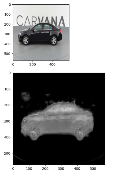
First of all, thank you so much for being patient with me. I am really enjoying learning more with this personal project. My network training saturates at 0.5 dice loss. The colab notebook can now be view by you and have shared the link in DM.
I infered a sample instance after training the model which saturated at 0.5 dice loss. Below is the visualization of the instance