GPU Performance Bottleneck: What are the possible causes?

Two identical models implemented in different ways have discrepant performances. How to identify the possible causes and how to solve them?

From a learning perspective, I’m implementing a Variational Autoencoder in order to achieve a performance close to the implementation of AutoencoderKL. However, my implementation is not performing properly and I’m looking for help to understand the possible reasons for the bottleneck.

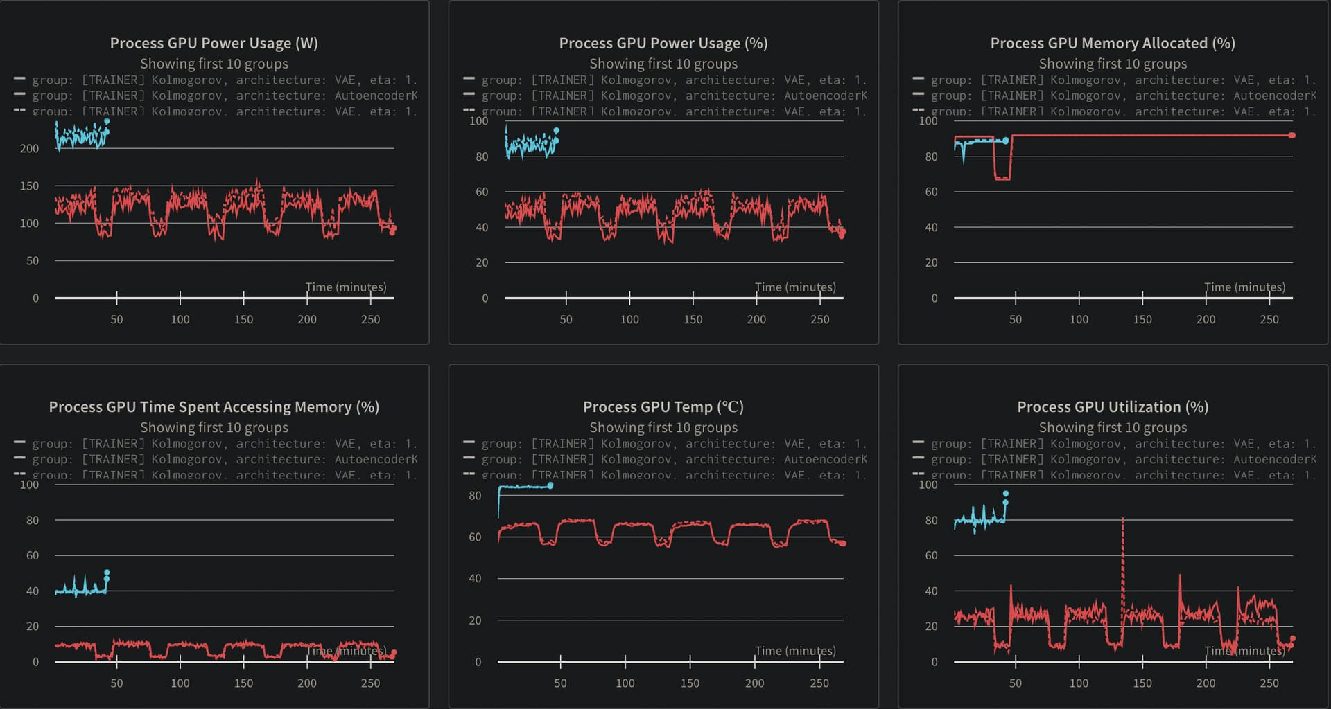
For context, here’s a comparison of GPU usage for the same run with the two different models. Although they are similar in terms of memory consumption, as the models have the same architecture, the use of the GPU in my implementation falls short. Furthermore, it is noted that, for the same number of epochs, the training time is 5-6x worse than the benchmark.

In addition, I profiled both runs with torch.profiler.profile. I have a lot of data in tensorboard from this profiling that I can share, I’m just not sure what information to share that might contribute to this diagnosis. If you have any suggestions on which views would be interesting, let me know and I’ll share them.

As a new user, I can only share one media in the post, however, I noticed a significant discrepancy when I look at the DIFF view on the tensorboard between both models. In this view, my model has a much higher execution than the benchmark.

Finally, both models share all training code, which includes DDP, AMP, and gradient norm clipping. Here is the code that is being used for training:

total = 0.
self.model.train()
self.train_data.sampler.set_epoch(epoch)
scaler = torch.cuda.amp.GradScaler()

for images, _ in data:
    self.optimiser.zero_grad(set_to_none=True)
    images = images.to(self.device)
    with torch.autocast(device_type='cuda'
                        if torch.cuda.is_available() else 'cpu',
                        dtype=torch.float16):
        if self.architecture == "AutoencoderKL":
            posterior = self.model.module.encode(images).latent_dist
            z = posterior.sample()
            recon = self.model.module.decode(z).sample
        else:
            recon, posterior = self.model(images)
        loss = (self.criterion()(recon, images) +
                self.eta * posterior.kl().sum())
    scaler.scale(loss).backward()
    scaler.unscale_(self.optimiser)
    torch.nn.utils.clip_grad_norm_(self.model.parameters(), 1.0)
    scaler.step(self.optimiser)
    scale = scaler.get_scale()
    scaler.update()
    self.optimiser.zero_grad(set_to_none=True)
    total += loss.item() * images.size(0) / len(data.dataset)
    del loss

if self.scheduler is not None:
    if not scale > scaler.get_scale():
        self.scheduler.step()

return total

Thanks in advance for the support. I am available for further clarification.

I usually take a look at the Trace view in the pytorch profilder visualization. I use record_shapes, profile_memory, and with_stack for the profiler in general. The trace view should highlight which parts of the code take long to execute. Does that help in your case?

1 Like

@fabian_schutze, I appreciate your response and indeed those are the settings I’ve used when profiling. I’ve taken a look at the trace view and tried to compare both models for the same profiler step, however, since I’m not much knowledgeable in this matter, I’m not sure if I spotted the issue.

It was not possible to observe much difference in the wall duration between the two models. As for the stream, on the other hand, I noticed that in my implementation there are two tags, stream 7 and stream 78, while in the benchmark, it was only possible to observe one: stream 7. Below is an image illustrating the view of my implementation.

Do you think this could be the reason for the discrepancy? If so, is there any reference that I could seek to better understand this process and perhaps some alternatives to this divergence?

Hi,

I would not concentrate yet on the streams, I would concentrate first on verifying the 5-6 times slower training in the Trace view. You should see that for the network with the slower training time that one training step (wrapped inside the profiler) takes much loner than the other one. Once you have identified these difference in duration, you can drill down and try to infer the cause for the discrepancy.

1 Like

@fabian_schutze, once again I appreciate your response. Isolating just one profiler step, which encapsulates a training step, it can be seen that there is no significant difference between the two implementations. However, I noticed completely unexpected behaviour.

I’m using wandb.ai as a logging tool and, for profiling, I’ve disabled its functionality via export WANDB_MODE=‘disabled’. When re-enabling the wandb, the initial discrepancy is observed during runtime, as initially reported. These results are also in line with just measuring the execution time of each training and validation function call in the code using time.

The image below contains the frame view of the results when disabled - the enabled one for my implementation is so expensive that its visualization doesn’t load. The first column represents the benchmark, while the second column represents my implementation.

In a summarized way, below are the results considering only the measurement of the execution of the training and validation functions for 1 epoch of these experiments and, as can be seen, they are in line with the results of the frame view.

Benchmark 			   WANDB_MODE='disabled'	    WANDB_MODE='enabled'
[GPU: 1] Training: 			382.7056 seg				636.9944 seg
[GPU: 0] Training: 			383.5272 seg				639.3160 seg
[GPU: 1] Validation: 		49.8034 seg					49.91465 seg
[GPU: 0] Validation: 		49.6792 seg					49.83615 seg

Implementation		   WANDB_MODE='disabled'	   WANDB_MODE='enabled'
[GPU: 1] Training: 			393.1595 seg				1953.5220 seg
[GPU: 0] Training: 			393.1553 seg				1953.4988 seg
[GPU: 0] Validation: 		42.5918 seg				    640.98976 seg
[GPU: 1] Validation: 		42.6761 seg				    619.39889 seg

My hypothesis, therefore, was that this drop in performance is linked to other parameters that are logged by wandb, such as gradients and model parameters. After disabling this wandb functionality via wandb.watch(log=None), I completely restored the performance of my implementation and it is now equivalent to the benchmark.

Finally, it seems that differences in model implementation - such as the choice of nn.Sequential, nn.ModuleList, etc - have a significant effect on the logging of gradients and parameters in the wandb.

1 Like