How can I display a test image and display the mask for it based on my trained model?

Neda · December 25, 2018, 12:41pm

I am wondering how I can test the trained model for semantic segmentation and visualise the mask for the test image. There is an example for classification problem in Pytorch but couldn’t find any obvious example for the segmentation.

I found this page that test the network, but it’s for classification problem.

I did manipulate it for segmentation application like below but now sure am I doing it right?

  model.eval()
    total = 0
    correct = 0
    count = 0
    #iterate through test dataset
    for data in (test_loader):
                
                t_image, mask = data
                t_image, mask = t_image.to(device), mask.to(device)
                with torch.no_grad():

                    outputs = model.forward(t_image) 
                    ps = torch.exp(outputs)
                         
                    _, predicted = torch.max(outputs.data, 1)  # Find the class index with the maximum value.
                    # We can use the PyTorch.eq() function to do this, which compares the values in two tensors and if they match, returns a 1. If they don’t match, it returns a 0
                    # By summing the output of the .eq() function, we get a count of the number of times the neural network has produced a correct output,
                    # and we take an accumulating sum of these correct predictions so that we can determine the overall accuracy of the network on our test data set.
                    total += mask.size(0)
                    correct += predicted.eq(mask.data).sum().item()
                    count +=1                
                    print("Accuracy of network on test images is ... {:.4f}....count: {}".format(100*correct/total,  count ))

the first question is why it used only forward here outputs = model.forward(t_image)?

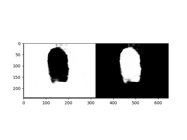
And the second question is how can I visualise the output of the test, for example, how can I display a test image and drow the mask for it based on my trained model? Is there any example for this? Thank you in advance.

tom · December 25, 2018, 6:38pm

Because they haven’t asked here to be told that you should use output = model(t_image).
More seriously, you would not call .forward unless you have a very good reason to not call the model itself (i.e. you tried that, it failed, you know why it failed and why calling .forward is better and, personally, I’d ask here about why calling the model won’t work).

I use pyplot a lot

# magic line only if you use Jupyter
%matplotlib inline
from matplotlib import pyplot
...
# assuming mask is batch x h x w and we want the first
pyplot.subplot(1, 2, 1) # have two plots in 1 row two columns, first plot
# assuming im is batch x channel x h x w and channel is RGB
pyplot.plot(im[0].detach().cpu().permute(1, 2, 0))
pyplot.subplot(1, 2, 2) # second plot
pyplot.plot(mask[0].detach().cpu())

Best regards

Thomas

Neda · December 25, 2018, 8:00pm

@tom thank you. calling the model is working.

In pyplot.plot(mask[0].detach().cpu()) I think you did plot the current mask (ground truth) which is already in the dataset. is that right?

Maybe I didn’t ask my question clearly. I wanted to test the model and display a test image from test_loader and visualise a predicted segmentation mask for this test image to find out is model learned anything or not. (for example like Predicted Mask(U-Net) in fig 3 in this paper.

tom · December 25, 2018, 8:36pm

Hi,

sorry, I didn’t adapt it well to your specific code. If just using predict in place of mask (based on accuracy involving predicted.eq(mask.data)) doesn’t work, what’s the shape of predict?

Best regards

Thomas

Neda · December 26, 2018, 2:59pm

@tom predict size is torch.Size([1, 240, 320]) and image size is torch.Size([1, 1, 240, 320])

tom · December 28, 2018, 1:18pm

Then the above recipe should work for predict in place of mask.

Best regards

Thomas

Neda · December 29, 2018, 3:53pm

I still couldn’t figure out how can I visualise the output of network after training. This code will visualize the raw output but I don’t know how can I display all dim of image, at the moment will display only one channel in plt.imshow(outputs[0,0,:,:].detach().cpu()) while the shape is #print(outputs.shape) # torch.Size([1, 2, 240, 320]) it is the same issue with plt.imshow(t_image[0,0,:,:].detach().cpu()) while the shape is #print(t_image.size()) # torch.Size([1, 1, 240, 320])

model.eval()
    total = 0
    test_loss = 0
    correct = 0
    count = 0
    #iterate through test dataset
    for vi, data in enumerate(test_loader):
                
                t_image, mask = data
                #print(t_image.shape) # torch.Size([1, 1, 240, 320])
                t_image, mask = t_image.to(device), mask.to(device)
                with torch.no_grad():

                    outputs = model(t_image)
                    #print(outputs.shape) # torch.Size([1, 2, 240, 320])
                    test_loss += criterion(outputs, mask).item() / len(test_loader)

                    pr = torch.exp(outputs) # get the exp of output and will give the probability map of outputs
                    # The outputs are energies for the 2 classes.
                    # Higher the energy for a class, the more the network thinks that the image is of the particular class. So, let’s get the index of the highest energy:     
                    _, predicted = torch.max(outputs.data, 1)  
                    
                    total += mask.size(0)
                    correct += predicted.eq(mask.data).sum().item()
                    accuracy = 100 * correct / total
                    predict = predicted.eq(mask.data)
                    #print(predict.shape) # torch.Size([1, 240, 320])
                    count +=1                
                    print(count, "Test Loss: {:.3f}".format(test_loss), "Test Accuracy: %d %%" % (accuracy))

    
    plt.figure()
    plt.subplot(1, 4, 1)
    #print(outputs.shape) # torch.Size([1, 2, 240, 320])
    plt.imshow(outputs[0,0,:,:].detach().cpu())
    plt.title('DL raw output')
    plt.subplot(1, 4, 2)
    plt.imshow(predict.detach().cpu().squeeze())
    plt.title('DL prediction')
    plt.subplot(1, 4, 3)
    plt.imshow(mask.detach().cpu().squeeze())
    plt.title('ground truth')
    plt.subplot(1, 4, 4)
    #print(t_image.size()) # torch.Size([1, 1, 240, 320])
    plt.imshow(t_image[0,0,:,:].detach().cpu())
    plt.title('original input image')

@ptrblck Could you please help to sort out this issue? I did try permute(1, 2, 0)) but couldn’t solve the issue

ptrblck · December 30, 2018, 12:42pm

I’m not sure, why it’s not working.
If you would like to visualize both probability maps for the two classes, your code should work:

plt.figure()
plt.imshow(torch.exp(outputs[0,0,:,:]).detach().cpu())  # plot class0
plt.figure()
plt.imshow(torch.exp(outputs[0,1,:,:]).detach().cpu())  # plot class1

What is your output currently showing?

Neda · December 30, 2018, 3:16pm

@ptrblck thank you for the probability map. You helped me before for the probability map of output, and it’s done. I wanted to visualise the prediction results from the test_loader, the mask (ground truth), and an original input image. I am wondering why my original input image doesn’t look grayscale image. Am I doing something wrong?


     #test model
    model.eval()
    total = 0
    test_loss = 0
    correct = 0
    count = 0
    #iterate through test dataset
    for vi, data in enumerate(test_loader):
                
                t_image, mask = data
                #print(t_image.shape) # torch.Size([1, 1, 240, 320])
                t_image, mask = t_image.to(device), mask.to(device)
                with torch.no_grad():

                    outputs = model(t_image)
                    #print(outputs.shape) # torch.Size([1, 2, 240, 320])
                    test_loss += criterion(outputs, mask).item() / len(test_loader)

                    pr = torch.exp(outputs) # get the exp of output and will give the probability map of outpus
                    # The outputs are energies for the 2 classes.
                    # Higher the energy for a class, the more the network thinks that the image is of the particular class. So, let’s get the index of the highest energy:     
                    _, predicted = torch.max(outputs.data, 1)  
                    
                    total += mask.size(0)
                    correct += predicted.eq(mask.data).sum().item()
                    accuracy = 100 * correct / total
                    predict = predicted.eq(mask.data)
                    #print(predict.shape) # torch.Size([1, 240, 320])
                    count +=1                
                    print(count, "Test Loss: {:.3f}".format(test_loss), "Test Accuracy: %d %%" % (accuracy))

    
    plt.figure(figsize=(11,4))
    plt.subplot(1, 3, 1)
    plt.imshow(predict.detach().cpu().squeeze())
    plt.title('DL prediction')
    plt.subplot(1, 3, 2)
    plt.imshow(mask.detach().cpu().squeeze())
    plt.title('ground truth')
    plt.subplot(1, 3, 3)
    #print(t_image.size()) # torch.Size([1, 1, 240, 320])
    plt.imshow(t_image.detach().cpu().squeeze())
    plt.title('original input image')

InnovArul · December 30, 2018, 3:24pm

you could try to use grayscale colormap.

Neda · December 30, 2018, 4:38pm

@InnovArul thank you. Yes cmap = ‘gray’ display the original image as grayscale.

Neda · January 4, 2019, 1:50am

@ptrblck one more question here, if I visualize the probability of output same as your example

plt.figure()
plt.imshow(torch.exp(outputs[0,0,:,:]).detach().cpu())  # plot class0
plt.figure()
plt.imshow(torch.exp(outputs[0,1,:,:]).detach().cpu())  # plot class1

it return a figure which is different with the figure that visualize by following example

    output = model(t_image)
    prob = torch.exp(output)
    prob_imgs = make_grid(prob.permute(1, 0, 2, 3))
    prob_imgs = prob_imgs.detach()
    plt.imshow(prob_imgs.permute(1, 2, 0))

what is cause to be different in these example, is it because of make_grid? because permute is just swap the first (batch size) and second dimensions (number of classes).
this image is from second example, for the first example the zeros value in figures will be 1 and 1 converted to zeros. (black and white will swap). which way is correct way to do this? thank you in advance
train_exp3

ptrblck · January 4, 2019, 10:01pm

I guess the difference in the visualizations is because make_grid created a “color” image (i.e. a tensor with 3 channels), which matplotlib apparently treats differently than an image without any channel dimension.
As long as the values and visualizations are consistent, you could just stick to the approach which you like more.

noornk · June 28, 2019, 2:23am

Why do we have to plot the mask in two figures? I don’t get this.
And how are we supposed to calculate the precision of the mask? I mean the area of intersection.

ptrblck · June 28, 2019, 9:47am

The code plots the probability maps for both classes, not the mask.
If you are only interested on a single class, you can of course just plot the corresponding prediction.

You could use the IoU implementation or a dice score.

noornk · July 12, 2019, 2:55am

Dear @ptrblck sorry for asking so many questions.
I still have trouble understanding this. The input of the network, for a binary class, is a [1, w, h] image. The prediction is [1, 2, w, h] (assuming the batch size is one), and the mask(ground truth) is [1, w, h]. I have to main questions:

How is the loss computed? the loss should get each cell’s value (which 0 or 1), and compare it to the mask values(again 0 or 1).
How to get the final predicted mask, in terms of an image? the output is class probability, then how am I suppose to get 0 or 1?

ptrblck · July 12, 2019, 10:40am

If you are using nn.CrossEntropyLoss (or nn.NLLLoss) for binary classification, each channel of the output will correspond to the logits (or log probabilities) of the class index.
Have a look at the CrossEntropyLoss docs to see the applied formula.
As you can see, the target will be used as an index to get the output logit, which corresponds to this target.

In the case of a binary classification, you can also use nn.BCEWithLogitsLoss, which would then expect an output of [batch_size, 1, h, w] and a target of the same shape.

If you want to get the prediction in terms of class indices, you can call preds = torch.argmax(output, 1) in the former case or use a threshold, if you are using nn.BCEWithLogitsLoss e.g.:
preds = torch.sigmoid(output) > 0.5.

noornk · July 12, 2019, 1:31pm

Thank you so much for your reply.
My output is in the shape of [batch_size, 2, h, w], and target is [batch_size, g, w], so I tried to use nn.CrossEntropyLoss, but I’m getting this error:

RuntimeError: “host_softmax” not implemented for ‘Long’

And when my output is [batch_size, 2, h, w], take for example these two cells: [0, 0, 10, 10] and [0, 1, 10, 10]. Shouldn’t the values complement each other? because the cell is in either class?

ptrblck · July 12, 2019, 1:43pm

Could you post the code snippet which throws this error?
Are you passing the model output as float and targets as long to nn.CrossEntropyLoss?

Since they represent logits, you won’t see any pattern there.
However, you could apply a softmax on dim1 and see the corresponding probabilities in each channel for the sake of debugging.

noornk · July 12, 2019, 1:52pm

Yeah. fixed it! However, now in the middle of training all the outputs become zero.