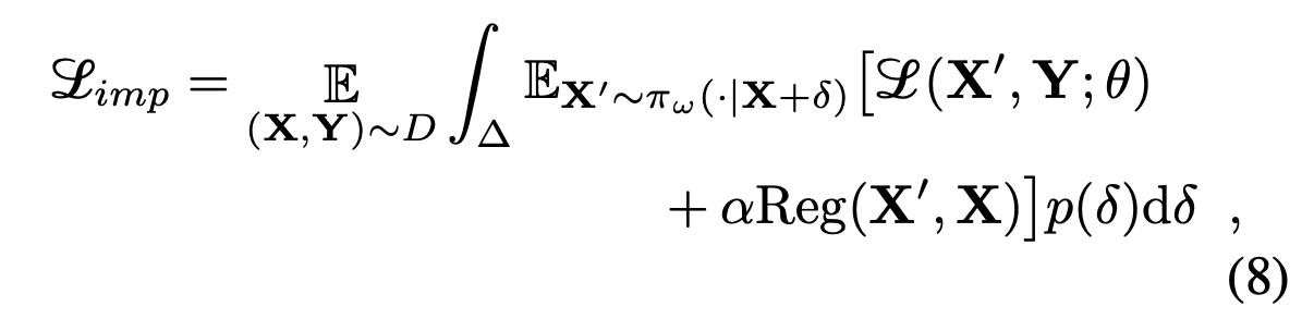
The loss function requires to integrate over the whole perturbation space for every input image. Each perturbation delta is a vector.
My questions:
Since the space of perturbation is continuous with infinite examples, it seems we can only sample finite number of perturbation to approximate the integral, is it correct?
If n perturbations are sampled for approximating the integral. How do we implement and approximate the above loss function? changing the integral to summation over the n perturbations sampled? How to implement it as batch processing?
Overall, my question is how to approximate integral over a continuous multi-dimensional space and how to implement the approximation in an elegant vectorization way? Any ideas and suggestions are welcomed. Thanks to the community!
As you guessed, you can only approximate the integral as a sum, not that the integral you are dealing with is also an expectation, so all your formula can be seen as the expectation over X,Y and \delta. In my opinion, you can create a loader over your original dataset, and that yields in addition to X and Y the perturbed X’. Then you can do the rest of the training as usual.
One other thing that seems strange in you case, is that you model $\pi_{\omega}$ seems to be non-deterministic. However I think in practice I think this will be a neural network, so the second expectation on X’ can be ignored, and you can just compute the loss using the output of $\pi_{\omega}$.
To summarize, you need to:
Each sample consists of X_{i}, y_{i} and a random $\delta$ generated on the fly, when reading the sample.
When you get a batch of X_{1:B}, y_{1:B} and \delta_{1:B}, you compute X’ = \pi_{\omega}(X+\delta).
You use X’ as your new input to the classification model you are training, i.e., the model labeled with $\theta$, and you compute the first part of the loss as for any classification problem, and you add the regularization term.
Thank you so much, @omarfoq! It solves my question of implementation and I guess that’s how it is approximated in practice. Got a couple follow-up of math notations in this kind of equations.
“your formula can be seen as the expectation over X,Y and \delta” . I understand this as following: it’s an integral of a 3 random variables (X, Y, delta) function. Here the sense of expectation comes from integral operation. My question is what the two E notations(E_{(X,Y)}~D and E_X^{\prime}~pi_{\omega}) are literally used for in the equation. If the integral operation gives the meaning of expectation, what’s the meaning of having the first E in the beginning of the equation, if we omit the first E, what goes wrong? Similar question for the second E. If the second E is not ignored, does it mean there should be another integral over X^{\prime} on [L + Reg]? Thanks.
Expectation is indeed a Lebesgue integral. When we write $\mathbb{E}{(X,Y) \sim D} f(X,Y)$ it can be understood as $\int{X, Y \in \mathcal{X} \times \mathcal{Y}} f(x,y) p_{D}(x, y) dx dy$ where $\mathcal{X}$ ad $\mathcal{Y}$ are the input and output sets and $p_{D}(x,y)$ is the density of $(x, y)$. So the first expectation in your equation, means that you integrate over all possible samples weighted with a density function of the distribution $D$. Note that in practice, we don’t know this density function, so the expectation term is approximated by an empirical average, this is why we take the average over all elements in the dataset.
Some parts of what I said here an not 100% accurate, I need far more space and notation to write the exact definitions, but I hope my answer was clear.
Great explanation! Let me rephrase this approximation strategy:
To approximate the first E, we iterate over all (X, Y) in dataset
To approximate the integral while ignoring the second E, we give each (X, Y) a random delta on the fly. This means each example will be paired with multiple deltas during the whole training process with multiple epochs. Overall, it approximates the integration over the space of upper cased Delta for each (X, Y).
Then, we do it in batches. At each batch, we use the average L_{imp} to back-propagate. I hope I didn’t misunderstand your explanation. Thanks.