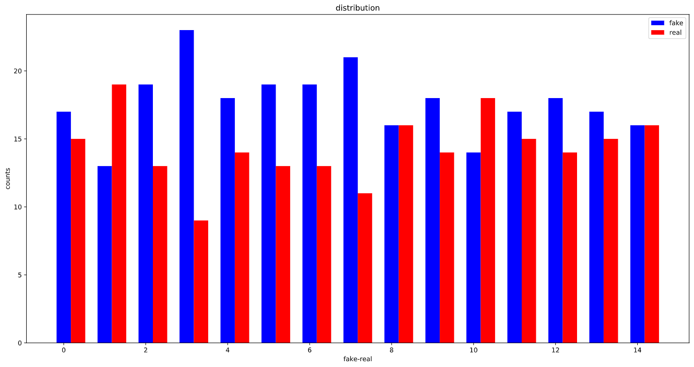
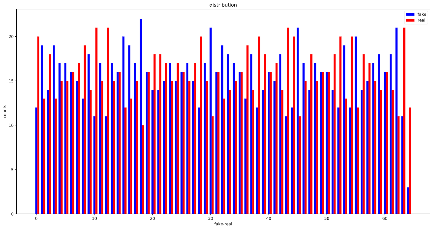
OK, looks like, the WeightedRandomSampler is correctly set up as the distribution of labels in each batch is considerably more balanced than before :
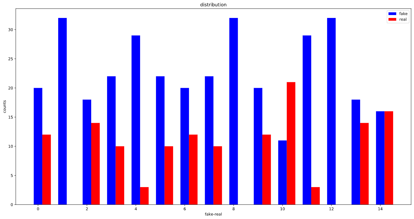
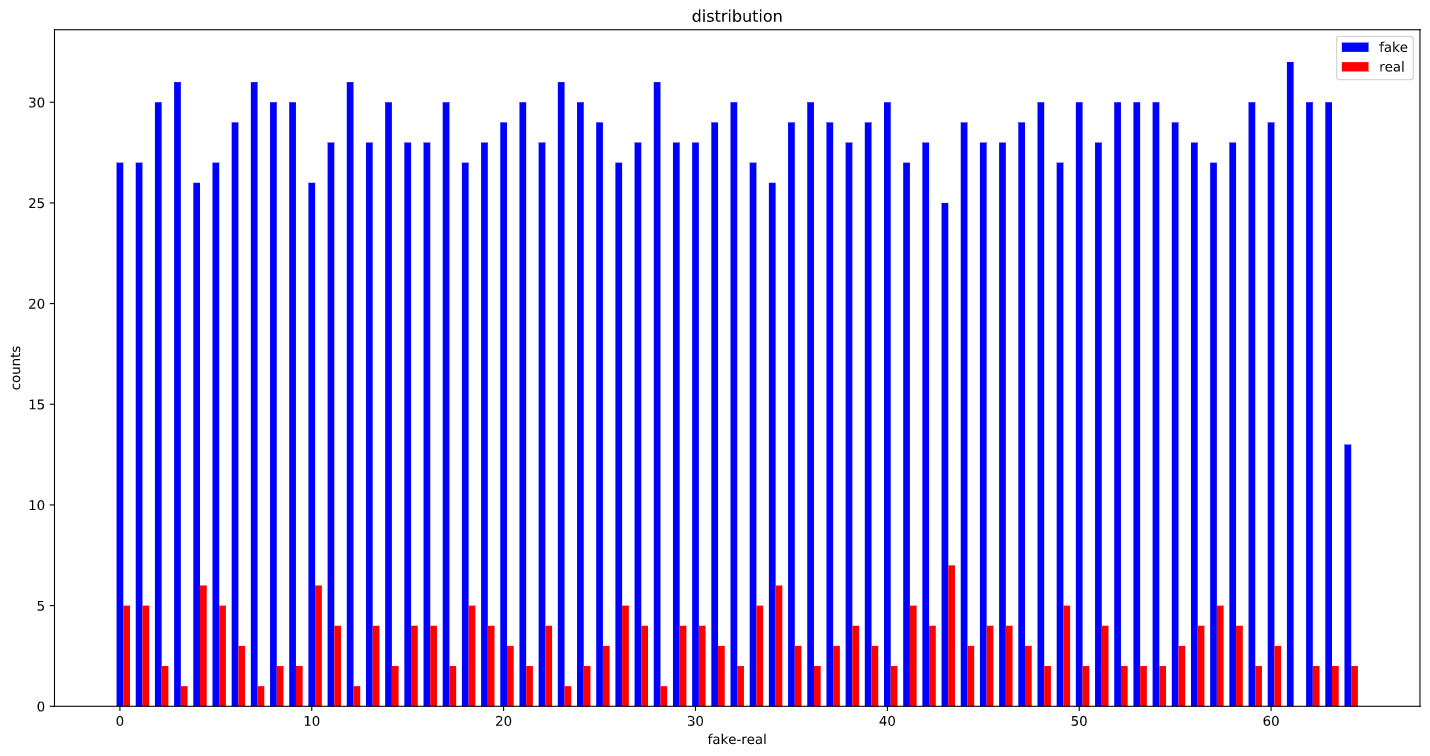
Before using the WeightedRandomSampler:
After using WeightedRandomSampler:
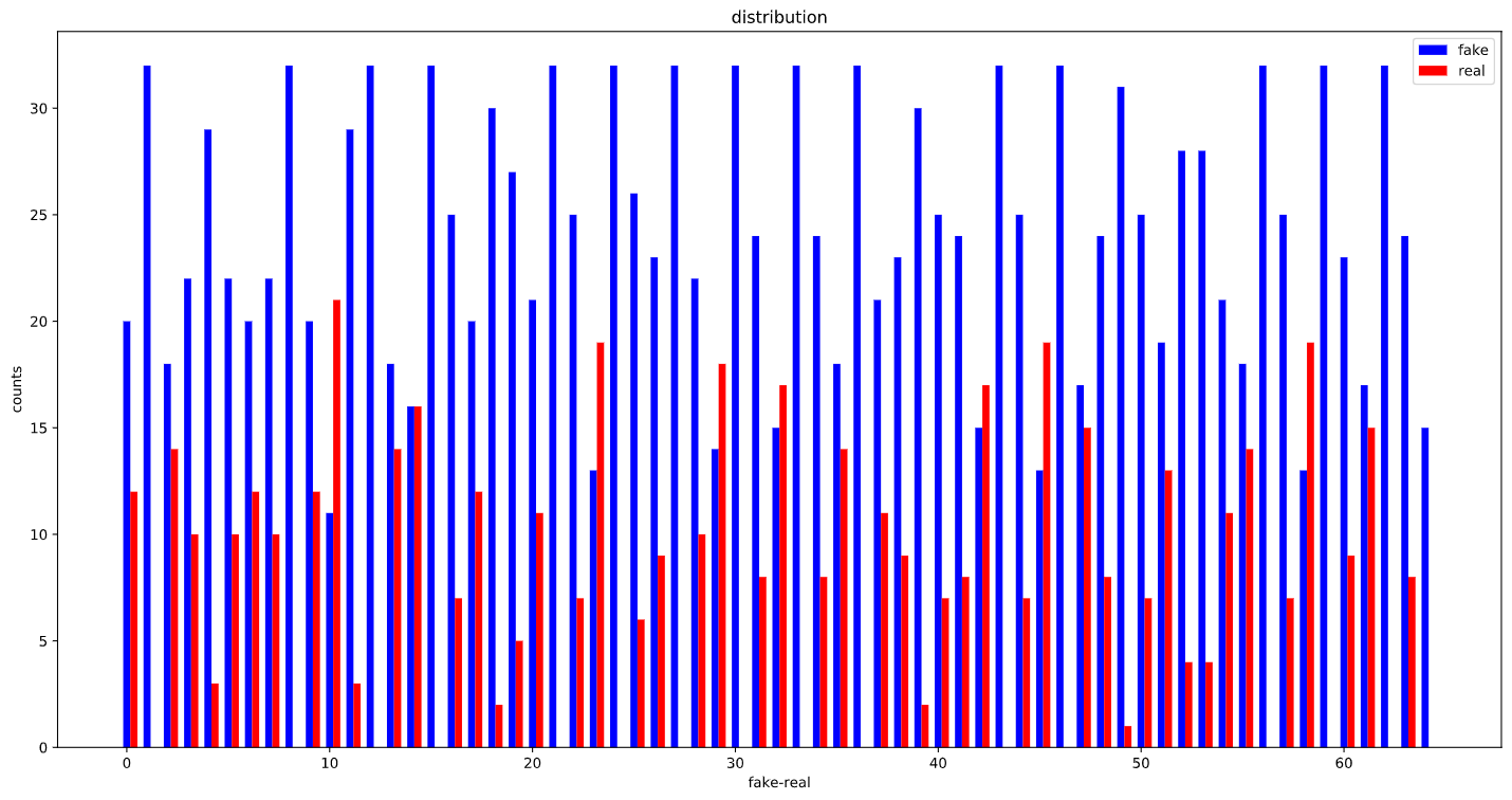
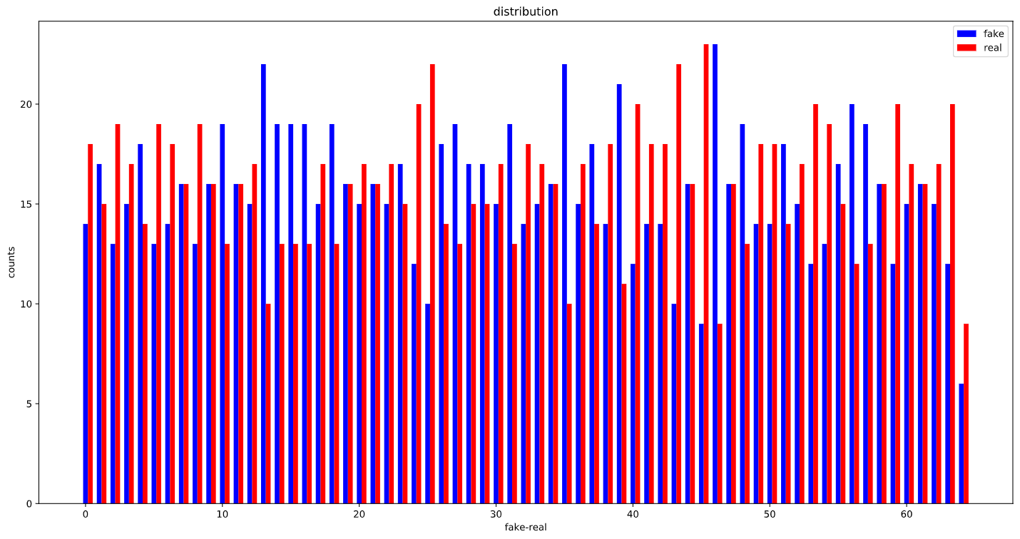
The whole training set:
Before:
After :
So I guess I got my answer to the first question.
For the second question concerning the class_weight I noticed something strange:
class_weights = 1./torch.Tensor(class_sample_counts)
results in this :
but when I calculated the class_weights like this :
# get list of all labels
train_targets = dt_train.get_labels(True)
labels, counts = np.unique(train_targets, return_counts=True)
class_weights = [sum(counts)/c for c in counts]
This is the result :
No wonder I was getting skewed results when using WeightedRandomSampler.
And for the second question : the batch_size vs the length of weighted_labels, the answer is, the length of weighted labels is necessary as it provides you with the whole data you have. if you use batch_size, you’ll only be using the batch_size number of data and thats done in one go! so the length of weighted_labels (or the number of labels) should be sent as the right number of samples ( hence the name num_samples)!
also here is the snippet of code I wrote for the batch distribution visualization that you see here. it might come in handy for someone out there specially if they are not well versed with plotting like me.
Pardon me for my lack of experience with matplotlib and plotting in general! :
zeros = []
ones = []
for img, label in dl_train:
    lbl = list(label.detach().numpy())
    res, cnts = np.unique(lbl, return_counts=True)
    if len(res) == 2:
        zeros.append(cnts[0])
        ones.append(cnts[1])
    else:
        if res == 0:
            zeros.append(cnts[0])
            ones.append(0)
        else:
            zeros.append(0)
            ones.append(cnts[0])

num_samples = len(zeros)
plt.figure(figsize=(15, 8))
plt.bar(np.arange(len(ones[:num_samples])), zeros[:num_samples], color='b', label='fake', width=0.35)
plt.bar(np.arange(len(ones[:num_samples]))+0.35, ones[:num_samples], color='r', label='real', width=0.35)
plt.xlabel('fake-real')
plt.ylabel('counts')
plt.title('distribution')
plt.legend()
plt.tight_layout()
plt.show()
also concerning the weights for losses see this