How to use autograd in the C++ api to compute a gradient of a multivalued function?

[tmaric]

I would like to calculate y = sin(x), where x is a vector of length N and compute the corresponding derivative vector y’ = (dy_i / dx_i), i = 1,2,3,…,N using autograd.

This is what I ended up doing:

    // Input vector x 
    auto x = torch::linspace(
        0, M_PI, 100, torch::requires_grad()
    ); 

    // sin(x) as a vector-valued function 
    auto sinx = torch::sin(x); 
    // backpropagate so that the gradient value is stored at x 
    sinx.backward(torch::ones_like(x));
    // x.grad() is dsin(x_i)/dx_i for some reason and not sinx.grad() 
    auto xgrad = x.grad(); 
    // sin'(x) = cos(x) for comparison
    auto cosx = torch::cos(x); 

and it seems to work:

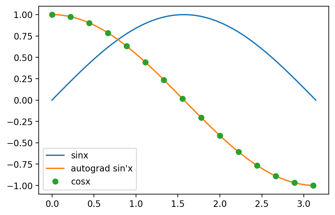
Is this correct and are there other ways (torch::autograd::grad) to calculate the gradient?

I have two questions.

1. Why do I have to give the argument torch::ones_like(x) to the backward function of sinx ? I understand the backpropagation in a network, there’s the output given by the model, and the difference between the output and the target is proportional to the gradient at this layer with respect to the weights and biases, this is used to correct the network parameters, etc. Here there is simply x → sin(x),there aren’t any weights and biases in this “network” (AD graph).

2. x → sin(x) is an acyclic directed graph, so why is the gradient of sin(x) stored at x? Why not at the sinx node? x.grad() somehow doesn’t intuitively mean sin’(x). Is x.grad() here the gradient of the root node (sinx) with respect to x, or did I misunderstand something?

[albanD]

Hi,

I think the best way to see what happens here is to write the Jacobian of your function and see what happens when you do the vector jacobian product (backward pass).
For your sin function, it just applies the sin element-wise to the input. So the Jacobian matrix is a diagonal matrix with on each diagonal element being the gradient of a single y_i wrt to x_i.

Now when you do the backward pass with a vector of all ones (from your torch::ones_like(x)). Then you do a matrix product between a vector of ones and a diagonal matrix.
This will return to you a vector containing the diagonal of the matrix.
And this new vector happens to be exactly what you’re looking for.

Note that this won’t be true anymore as soon as your Jacobian is not diagonal anymore though!

[tmaric]

Thanks a lot for the hint! I thought that a full Jacobian is always computed by backward, as described in the documentation on Vector Calculus using autograd. Is there any documentation besides the source code of backward that describes the calculation of the Jacobian?

[albanD]

That documentation that you linked explicitly states that it computes a vector jacobian product

If you want to get the full jacobian in general, you will need to do as many backward as there are outputs to your function.
In the special case where it is diagonal though (like here), you can compute it in one go as done in your example.

[tmaric]

Cool, thanks!

So reading the line in the documentation linked above, that states

Equivalently, we can also aggregate Q into a scalar and call backward implicitly, like Q.sum().backward() .

This is just a trick to use the sum to have a real-valued output function and not vector-valued output function, and by doing so simplify the call to backward and populate grad objects with data?

[albanD]

Doing the sum() like that is the same as calling backward with a vector full of ones like you do.

But why it works is because it makes the overall function have a single output and so the overall jacobian has a single row. And multiplying it by a vector of [1] will return that row in one backward pass.

[tmaric]

I played a bit with torch::autograd::grad.

if x,y in R^3 and f = dot(x,y), then f : R^3 -> R.

f = x1y1 + x2y2 + x3y3

Now I want grad_x f (sensitivity of f with respect to x), which is a scalar by vector derivative, and I expect to get

grad_x f = [ df / dx1 df/dx2 df/dx3 ]^T = [y1 y2 y3]^T

which makes sense because dot(x,y) is linear in x, and y is kept constant with grad_x f.

Here’s the code with x = y,

    auto x = torch::linspace(0, 1, 3, torch::requires_grad()); 
    auto y = torch::linspace(0, 1, 3, torch::requires_grad()); 
    auto f = dot(x,y); 

    std::cout << "x = \n" << x << std::endl;
    std::cout << "y = \n" << y << std::endl;
    std::cout << "f = dot(x,y) = " << f << std::endl;
    
    auto grad_f = torch::autograd::grad(
        {f}, {x}, {torch::ones_like(x)}
    );

    std::cout << "grad_f = \n" << grad_f << std::endl; 

and the output for grad_f is

x = 
 0.0000
 0.5000
 1.0000
[ CPUDoubleType{3} ]
y = 
 0.0000
 0.5000
 1.0000
[ CPUDoubleType{3} ]
f = dot(x,y) = 1.25
[ CPUDoubleType{} ]
grad_f = 
 0.0000
 1.5000
 3.0000
[ CPUDoubleType{3} ]

which is not y, why? I seem to still be misunderstanding the J^T v calculation done in autograd.

[albanD]

Is the code you shared actually running? The grad output you give should be the same size as the output so f here and not x.
I am not sure why this actually runs without error…

[tmaric]

Yep, it’s running. The grad output should be the same as x… f is linear in x_i components. Gradient of a scalar function is a vector. Vector derivative of a scalar function is a vector…

[albanD]

The grad input should be the same size as the input (x here)
But the grad output should be the same size as the output (scalar f here)

[tmaric]

I think I have to read more about reverse mode automatic differentiation…

[albanD]

In this case, if you have your jacobian as a 2D matrix of size (nb_output, nb_input). And backward mode AD allows you to compute the vector jacobian product between a vector of size nb_output (grad output) with the jacobian to obtain a vector of size nb_input (grad input)

[tmaric]

If f = dot(x,y), then f = f (x,y), so the Jacobian should be J = [[df/dx1, df/dx2, df/dx3],[df/dy1, df/dy2, df/dy3]], if I want to compute the grad with output f and input {x,y}, right?

[albanD]

If f = dot(x,y), then f = f (x,y), so the Jacobian should be J = [[df/dx1, df/dx2, df/dx3],[df/dy1, df/dy2, df/dy3]]

No
To be able to write the jacobian as a 2D matrix, you need all inputs and outputs to be 1D Tensors.
So you will need to have a single output that is the concatenation of x and y. And then you can write the Jacobian as [[df/dx1, df/dx2, df/dx3, df/dy1, df/dy2, df/dy3]]

[tmaric]

Thanks! Can you point me to a source of documentation beyond what I’ve linked, that describes how exactly autograd::grad works? Should I go into the source code?

Here’s one more even simpler example

        std::vector<double> e {1, 0, 0}; 
        auto x = torch::from_blob(e.data(),3,torch::requires_grad());
        auto f = dot(x,x); 
        std::cout << "x = \n" << x << std::endl;
        std::cout << "f = dot(x,x) = " << f << std::endl;

        auto partial_f_x = torch::autograd::grad({f}, {x});
        std::cout << "partial_f_x = \n" << partial_f_x << std::endl; 

with the output:

[ CPUDoubleType{1} ]
x = 
 1
 0
 0
[ CPUDoubleType{3} ]
f = dot(x,x) = 1
[ CPUDoubleType{} ]
partial_f_x = 
 2
 0
 0
[ CPUDoubleType{3} ]

so if x in R^3, partial_x (dot(x,x))=2x.

[albanD]

@tmaric

Can you point me to a source of documentation beyond what I’ve linked, that describes how exactly autograd::grad works?

autograd.grad does reverse mode automatic differentiation (also called backpropagation), between the output and input that are given, using grad_output as first gradient (which default to 1 for scalar outputs).
You can find some work in progress doc here: Autograd mechanics — PyTorch master documentation

Should I go into the source code?

I don’t think that will help as it involves quite a lot of components and they interact in non obvious ways

so if x in R^3, partial_x (dot(x,x))=2x.

Yes that works as expected.
Note that for a first example, I would avoid re-using the same variable as it introduces implicit accumulations in the backward pass.

[tmaric]

Thanks a lot! I’ll read the in-progress doc around 20-30 times, maybe that’ll help hehe. I’ve read the PyTorch papers, one is pointing towards the AD book “Evaluating Derivatives
Principles and Techniques of Algorithmic Differentiation, Second Edition” by Andreas Griewank and Andrea Walther. I’ll try to pick up the reverse mode AD from there also.

I want to work with higher derivatives of the models, so I really must be 100% sure about what grad is doing and how to build up on that.

[pancras (Pancras Wang)]

Hello,my name is Pancras,I see you solve a related problem.So I want to ask you for help.

When I was training the model, loss always appeared nan. I don’t know what is the reason for nan? Can you help me analyze it? I used code monitoring and reported an error:RuntimeError: Function ‘CudnnBatchNormBackward’ returned nan values in its 0th output.looking forward to your reply