Implementing Tangent Prop Paper

[Zhihan_Yang]

I’m trying to implement an old paper: Tangent Prop - A formalism for specifying selected invariances in an adaptive network. .

For example, let’s consider the following regression problem. Suppose we have 1-dimensional input (x) and 1-dimensional output (y). In this case, the Jacobian matrix is just 1-by-1 (a scalar) that describes the derivative of y w.r.t. x. So far so good.

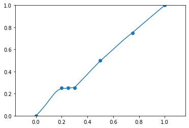
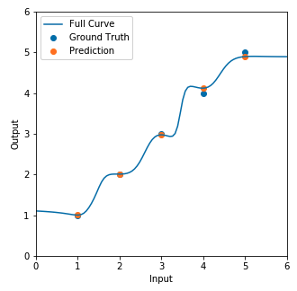
So we iteratively perform gradient descent for the regression sum-of-squares loss + adjustable parameter * the squared Jacobian. Ideally, when this loss is minimized, we get the learned function as the solid line (see diagram below) given that our neural net has enough capacity.

Without the squared Jacobian term, we would get the learned function as the dashed line (see diagram below).

However, what I described above fails when implemented in PyTorch as follows:

class Net(nn.Module):
    
    def __init__(self):
        super().__init__()
        
        self.main = nn.Sequential(
            nn.Linear(1, 100),
            nn.ReLU(),
            nn.Linear(100, 100),
            nn.ReLU(),
            nn.Linear(100, 1)
        )
        
    def forward(self, x):
        return self.main(x)

def get_model():
    model = Net()
    return model, optim.Adam(model.parameters(), lr=1e-3)

def sos(ypred, y):
    "Sum of squares loss"
    return torch.sum((ypred - y) ** 2)

def get_jacobian(net, x, noutputs):
    x.requires_grad = True
    y = net(x)
    grad_params = torch.autograd.grad(y, x, create_graph=True)
    return grad_params[0]

# just a straight line with slope 1 and intercept 0
data = [0., 0.25, 0.5, 0.75, 1.0] 
labels = [0., 0.25, 0.5, 0.75, 1.0] 

model, opt = get_model()
jacobian_losses = []
reg_losses = []
for i in range(100):

    ypred = model(torch.tensor(data).view(-1, 1))
    reg_loss = sos(ypred, torch.tensor(labels).view(-1, 1))
    reg_losses.append(float(loss))
    
    jacobian_loss = 0
    for x in [0., 0.25, 0.5, 0.75, 1.0]:
        jacobian = get_jacobian(model, torch.tensor([[x]]), 1)
        temp = torch.norm(jacobian) ** 2
        jacobian_loss += temp
    jacobian_losses.append(float(jacobian_loss))
    
    total_loss = reg_loss + 1e-1 * jacobian_loss
    
    total_loss.backward()
    opt.step()
    opt.zero_grad()

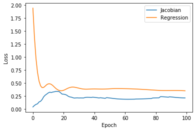
Here’s the losses plotted together:

plt.plot(jacobian_losses, label='Jacobian')
plt.plot(reg_losses, label='Regression')
plt.xlabel('Epoch'); plt.ylabel('Loss')
plt.legend()
plt.show()

Here’s the resulting regression line:

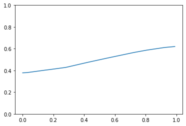
And we don’t see the polynomial-like regression line like we saw above in the figure given by the paper. Can anyone help point out my mistake(s)? I’ve tried multiplying Jacobian loss by a smaller weight but I still don’t see the curvatures.

[albanD]

Hi,

Given your loss, I guess it is expected that the curve does not look good right? It would. only look like your first image if the loss goes to 0 right?

Maybe your model is not expressive enough? Have you checked?

[Zhihan_Yang]

Hi albanD,

Thanks for the comment. You’re right: the loss plot reflects the fact that the curve does not look good.

So I tried a model with a higher capacity as follows and the curve still looks as bad.

Do you find any mistake in my get_jacobian function?

class Net(nn.Module):
    
    def __init__(self):
        super().__init__()
        
        self.main = nn.Sequential(
            nn.Linear(1, 100),
            nn.ReLU(),
            nn.Linear(100, 100),
            nn.ReLU(),
            nn.Linear(100, 100),
            nn.ReLU(),
            nn.Linear(100, 100),
            nn.ReLU(),
            nn.Linear(100, 100),
            nn.ReLU(),
            nn.Linear(100, 1)
        )
        
    def forward(self, x):
        return self.main(x)

[albanD]

Hi.

Changing the weight for the jacobian part to 100 makes it go to 0 nicely.
Similarly, putting it to a very low value makes the regular loss go to 0.

So it is an expression power of your model that fails to optimize both at the same time. Maybe try different activation? I am not sure that a relu network can do this task.

[Zhihan_Yang]

I tried the same model on the following data without increasing the expressive power of the model, yet the model was able to learn curvature with no problem (which is strange). I needed to increase the number of epochs for the model below to learn curvature, but adding the number of epochs did not work for minimizing regression loss + Jacobian loss.

Maybe there are some hidden mistakes in how I computed the Jacobian and the gradients?

Additional things I tried:

• I tried adding 3 more layers to my model and increasing the number of neurons per layer, but nothing worked.
• I tried changing the ReLU activations to Sigmoid activations. But for Sigmoids to perform well, BatchNorm1d was needed (probably due to vanishing gradients). However, if you look at my get_jacobian function, I’m passing through the network only ONE example, so BatchNorm1d would raise an error since batch-wise standard deviation can’t be calculated from a batch of one example.

data = [0, 0.20, 0.25, 0.30, 0.5, 0.75, 1.0]
labels = [0, 0.25, 0.25, 0.25, 0.5, 0.75, 1.0]

model, opt = get_model()
jacobian_losses = []
reg_losses = []
for i in range(300):
    
    ypred = model(torch.tensor(data).view(-1, 1).float())
    loss = sos(ypred, torch.tensor(labels).view(-1, 1))
    reg_losses.append(float(loss))
    
    loss.backward()
    opt.step()
    opt.zero_grad()

preds = model(torch.arange(-0.1, 1.1, 0.01).view(-1, 1)).view(-1).detach().numpy()
plt.scatter(data, labels)
plt.plot(np.arange(-0.1, 1.1, 0.01), preds)
plt.ylim(0, 1)
plt.show()

[Zhihan_Yang]

More than a year later, I decided to give this another go. I found that changing ReLU to Sigmoid / Softplus solved the issue. I was able to get the following plot: