Jacobian functional API batch-respecting Jacobian

I am hoping to get Jacobians in a way that respects the batch, efficiently

Given a batch of b (vector) predictions y_1,…,y_b, and inputs x_1 … x_b, I want to compute the Jacobians of y_i wrt x_i. In other words, I want a Jacobian of the output wrt input for each pair in the batch.

One might try the following:

import torch
import torch.nn as nn
# Load the experimental api 
# https://github.com/pytorch/pytorch/blob/master/torch/autograd/functional.py
from experimental_api import jacobian

in_dim = 5
batch_size = 3
hidden_dim = 2
out_dim = 10

f = nn.Sequential(nn.Linear(in_dim, hidden_dim), nn.Sigmoid(), nn.Linear(hidden_dim, out_dim))
x = torch.randn(batch_size, in_dim)

result = jacobian(f, x)
result.shape

torch.Size([3, 10, 3, 5])

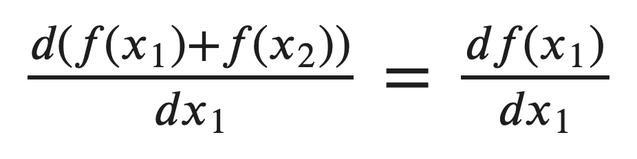
In this case, I wanted a result with shape (batch_size, out_dim, in_dim) = (3, 10, 5) but instead got extra dimensions. In fact, PyTorch is considering x as just one input matrix rather than a batch of several vectors. This leads to redundant calculation such as the derivatives of target 2 wrt input 1.

Clearly, I could do a loop like jacobian(f, x_row) for x_row in x but that would no longer use the GPU effectively. Can anyone propose an efficient solution?

4 Likes

Hi,

the functional API works at the autograd level and so is not aware of things like batch size.
Supporting this kind of use case is planned to be supported efficiently by using vmap with the functional API.

If you’re using a regular neural net, the simplest thing to do here is just to take the diagonal of the full jacobian you get (using dim1=0 and dim2=2). It does lead to useless computations but not that much.
In particular, if you call backward on your model (in any way) all the ops will work with the full batch size of the forward.
Your proposed solution will avoid these extra computations but might not be worth the loss in forward.

You can try them both and see the result. I would be interested to know which one is faster for your usecase?

1 Like

I have the exact same question as OP. I tested using torch.diagonal but because I also want to compute the second-order jacobian doing this using diagonal is extremely slow.

Here is the code I’m using

    def compute_u_x(self, x):
        self.u_x = torch.autograd.functional.jacobian(self, x, create_graph=True)
        self.u_x = torch.diagonal(self.u_x, dim1=0, dim2=2).permute(2, 0, 1)
        return self.u_x
    
    def compute_u_xx(self, x):
        self.u_xx = torch.autograd.functional.jacobian(self.compute_u_x, x)
        self.u_xx = torch.diagonal(self.u_xx, dim1=0, dim2=3).permute(3, 0, 1, 2)
        self.u_xx = torch.diagonal(self.u_xx, dim1=2, dim2=3)
        return self.u_xx

This will give me what I need, but it’s computing so many extra things it significantly slowed my training loop. I also made a version which isn’t vectorized that uses the torch.autograd.grad function which works exponentially faster than above. However, this method only works for scalar output functions, which is not what I need.

Computing a Hessian is expected to be slow I’m afraid.
Note that we have a function that computes the hessian directly in some cases that might help. But I don’t expect it to be much faster.

However, this method only works for scalar output functions

That’s the trick. If your function has a single input then the full Jacobian is recovered with a single backward pass and all the first order gradients become very easy to compute!

I was actually able to solve it. This works exponentially faster than using the jacobian and hessian methods + diagonalization. However, I suspect this still isn’t at peak efficiency due to the for-loop. Hopefully something like this can be parallelized and implemented in the future.

# Creates first and second order jacobian for vector function f
def second_order_jacobians(f, wrt, create_graph=True):
    jacobian_1 = []
    jacobian_2 = []
    for i in range(f.shape[1]):
        j1 = grad(f[:,i:i+1], wrt, create_graph=create_graph, grad_outputs=torch.ones(f[:,i:i+1].shape).to(f.device))[0]
        j2 = grad(j1, wrt, create_graph=create_graph, grad_outputs=torch.ones(j1.shape).to(j1.device))[0]
        jacobian_1.append(j1)
        jacobian_2.append(j2)
    jacobian_1 = torch.stack(jacobian_1, -1)
    jacobian_2 = torch.stack(jacobian_2, -1)
    return jacobian_1, jacobian_2

This works exponentially faster

You mean just faster right? I don’t see how that could be exponential…

And yes this will work fine as mentioned above. The only downside is that you now do many more forward passes. So depending on your application this will be better or not.

I was facing the same problem as OP and managed to get an elegant workaround using simple sum along the batch dimension of the original function. This means the result will be differentiated exactly as OP requested (just write it down). This approach is theoretically batch_size times faster than computing full jacobian and then using diagonal. I can see similar speedup in my calculations.

def batch_jacobian(f, x):
    f_sum = lambda x: torch.sum(f(x), axis=0)
    return jacobian(f_sum, x)

Note that it is necessary to permute the result to get the batch_dimension in front. In OPs case permute(1,0,2) will do the job.

The same trick can be applied for hessian and will bring even more significant speedup.

9 Likes

Very nice, didn’t think of it. Yields the exact same results as using a for loop, but runs much faster than the for loop.

Looks like a very nice workaround, but any explanation on why this can work?


Let me try this by myself.

One explanation in my mind is that the change of an instance in batch will contribute to the change of final sum result independently.

Formally,

1 Like

Indeed, since outputs can’t depend on any other inputs across the batch dimension, all cross-batch entries in the Jacobian are zero. So you’re still doing all the useless computations but now without a for-loop.

As mentioned above, the functional API works at the autograd level and so is not aware of things like batch size. You can think about this trick as working around this limitation by turning the batch of outputs into a sum of contributions and the batch of inputs into a single big example. Along the batch dimension, only the matching outputs and inputs will contribute a non-zero result.

Explicitly, for batches of input vectors getting transformed into batches of output vectors, the trick sums the outputs (batch_size, out) into (out) so that taking the derivative with respect to the “single big example” (batch_size, in) outputs a Jacobian with shape (out, batch_size, in). Permuting then gives you the Jacobian you want.

@mcbal Yes exactly. Although I do not agree with the statement

I do not really see the reason why the this would be the case. The test also indicate that this does not happen and the computation is much faster. Am I mistaken @mcbal ?

@martinsipka I could be wrong here, but I was under the impression that the speedup came from the parallelisation enabled by acting on the result of the sum across batches. The “batch-off-diagonal” terms are still present, but since the derivative across batches is zero they don’t yield a contribution to the sum. Here is a small code snippet to illustrate what I mean:

import torch
from torch import autograd, nn

bsz, dim_in, dim_out = 3, 5, 7

x = torch.randn(bsz, dim_in)
f = nn.Linear(dim_in, dim_out)

@torch.enable_grad()
def batch_jacobian(f, x):
    f_sum = lambda x: torch.sum(f(x), axis=0)
    return autograd.functional.jacobian(f_sum, x).swapaxes(1, 0)

print(batch_jacobian(f, x))

@torch.enable_grad()
def batch_jacobian_take_zeroth_output(f, x):
    f_sum = lambda x: f(x)[0]
    return autograd.functional.jacobian(f_sum, x).swapaxes(1, 0)

print(batch_jacobian_take_zeroth_output(f, x))

In this example, the first print statement returns the “batch-diagonal” Jacobian entries corresponding to (00, 11, 22), just like the snippet you posted earlier in this thread. The second print statement restricts the output to the zeroth element in the batch so that computing the Jacobian with respect to the full batch now includes some “batch-off-diagonal” entries (00, 01, 02). Only the zeroth element (00) in the batch contains non-zero entries, the other “batch-off-diagonal” entries (01, 02) are zero.