I am trying to do 10 fold CV with DNN. However, the loss curve change drastically when I do it in different ways. When I run the 10 fold CV in the fit method of the Module class, the loss curve has large fluctuations. But when I run the for loop on the KFolds object, and fit the training data separately, the loss curve is smooth and converges quickly.
Below is my code:
from sklearn.model_selection import KFold
#tune model in 10-fold CV:
#n fold CV on hc data:
nfold = 10
seed = 111
kf = KFold(n_splits=nfold, shuffle = True, random_state=seed)############################################# DNN (pytorch)
import torch
import torch.nn.functional as F
import torch.nn as nn
from torch.autograd import Variable
from torch.optim.lr_scheduler import ReduceLROnPlateauimport numpy as np
from sklearn.model_selection import train_test_split
from sklearn.model_selection import StratifiedShuffleSplit
import matplotlib.pyplot as plttorch.manual_seed(999) # reproducible
   def smooth(y, box_pts):
        box = np.ones(box_pts)/box_pts
        y_smooth = np.convolve(y, box, mode='same')
        return y_smooth
> def weights_init(m):
>     if isinstance(m, nn.Linear):
>         print('initialize weight...')
>         nn.init.xavier_uniform_(m.weight.data)
> class Model(nn.Module):
>
>     def __init__(self, n_hidden1=400, n_hidden2=150, n_hidden3=50,
>                  min_loss = .5, l_rate = .001, max_epochs = 10000):
>
>         super(Model, self).__init__()
>         self.n_hidden1 = n_hidden1
>         self.n_hidden2 = n_hidden2
>         self.n_hidden3 = n_hidden3
>         self.min_loss = min_loss
>         self.l_rate = l_rate
>         self.max_epochs = max_epochs
>
>
>     def build_layer(self, input_dim):
>
>         if input_dim<100:
>             print('4 layers .................')
>             # MD and FA:
>             n_hidden1 = 50
>             n_hidden2 = 20
>             n_hidden3 = 5
>
>             self.layer1 = nn.Linear(input_dim, n_hidden1)
>             self.layer2 = nn.Linear(n_hidden1, n_hidden2)
>             self.layer3 = nn.Linear(n_hidden2, n_hidden3)
>             self.layer4 = nn.Linear(n_hidden3, 1)
>             #self.layer5 = nn.Linear(5, 1)
>
>         elif input_dim<150:
>             print('5 layers .................')
>             # gray matter volume
>             n_hidden1 = 200
>             n_hidden2 = 100
>             n_hidden3 = 50
>
>             self.layer1 = nn.Linear(input_dim, n_hidden1)
>             self.layer2 = nn.Linear(n_hidden1, n_hidden2)
>             self.layer3 = nn.Linear(n_hidden2, n_hidden3)
>             self.layer4 = nn.Linear(n_hidden3, 20)
>             self.layer5 = nn.Linear(20, 1)
>             #self.layer6 = nn.Linear(5, 1)
>
>         elif input_dim<300:
>             print('5 layers .................')
>             # ALFF and ReHo
>             n_hidden1 = 200
>             n_hidden2 = 150
>             n_hidden3 = 50
>
>             self.layer1 = nn.Linear(input_dim, n_hidden1)
>             self.layer2 = nn.Linear(n_hidden1, n_hidden2)
>             self.layer3 = nn.Linear(n_hidden2, 1)
>             #self.layer4 = nn.Linear(n_hidden3, 20)
>             #self.layer5 = nn.Linear(20, 1)
>             #self.layer6 = nn.Linear(5, 1)
>
>         else:
>             print('6 layers .................')
>             self.layer1 = nn.Linear(input_dim, self.n_hidden1)
>             self.layer2 = nn.Linear(self.n_hidden1, self.n_hidden2)
>             self.layer3 = nn.Linear(self.n_hidden2, self.n_hidden3)
>             self.layer4 = nn.Linear(self.n_hidden3, 30)
>             self.layer5 = nn.Linear(30, 5)
>             self.layer6 = nn.Linear(5, 1)
>
>         self.sigmoid = torch.nn.Sigmoid()
>
>
>     def forward (self, x, **kwargs):
>
>         out = F.relu(self.layer1(x)) # activation function for hidden layer
>         #out1 = self.sigmoid(self.layer1(x))
>         #out1 = self.dropout(out1)
>
>         #out2 = F.relu(self.layer2(out1))
>         out = self.sigmoid(self.layer2(out))
>         #out2 = self.dropout(out2)
>
>
>
>         if x.shape[1]<100:
>             out = F.relu(self.layer3(out))
>             #out = self.dropout(out)
>
>             y_pred = self.layer4(out)
>
>         elif x.shape[1]<300:
>             out = self.sigmoid(self.layer3(out))
>             out = F.relu(self.layer4(out))
>             y_pred = self.layer5(out) # linear output
>
>         else:
>             out = self.sigmoid(self.layer3(out))
>             out = self.sigmoid(self.layer4(out))
>             out = F.relu(self.layer5(out))
>             y_pred = self.layer6(out) # linear output
>
>         return y_pred
>
>
>     def update_plot(loss_list, corr_list, loss_info):
>         corr_list_s = smooth(corr_list, box_pts = 100)
>         ax.clear()
>         ax.plot(range(epoch), loss_list,'r--', range(epoch), corr_list*10, 'g--',
>                range(epoch), corr_list_s*10, 'y--')
>         plt.ylim(0, 30)
>         plt.text(10, 30 , loss_info, fontsize=10)
>         fig.canvas.draw()
>
>
>     def fit (self, X, y,  max_loss = 10, tune_loss = False):
>         """
>         if tune_loss:
>         1. use 80% of data as training and 20% as test set to get the optimized number of epochs
>         2. reset the model use all the data to train the model.
>
>         Note: the tuned loss may not work better for independent validation data. As in K-fold CV, the training
>         and validation set are not independent. (e.g. larger mean value of training set indicates smaller mean
>         of the validataion set). It is recommend to first use tune_loss to explore the best min_loss, and run
>         the model again with tune_loss=False.
>         """
>
>         min_loss = self.min_loss
>         max_epochs = self.max_epochs
>
>         #torch.manual_seed(999)    # reproducible
>         self.build_layer(input_dim = X.shape[1])
>
>         criterion = nn.MSELoss()# Mean Squared Loss
>
>         optimizer = torch.optim.SGD(self.parameters(),
>                                     lr = self.l_rate,
>                                     weight_decay=1e-3,
>                                     momentum=0.9,
>                                     dampening = 0,
>                                     nesterov=True) #Stochastic Gradient Descent
>
>         scheduler = torch.optim.lr_scheduler.StepLR(optimizer, step_size=1000, gamma=.5)
>
>         if tune_loss==True:
>             print('optimizing loss value ...')
>             opt_loss_list = []
>
>             for train_index, test_index in kf.split(X, y):
>                 #print("TRAIN:", train_index, "TEST:", test_index)
>                 X_train, X_test = X[train_index], X[test_index]
>                 y_train, y_test = y[train_index], y[test_index]
>
>                 X_train_torch = Variable(torch.from_numpy(X_train))
>                 y_train_torch = Variable(torch.from_numpy(y_train))
>                 X_train_torch = X_train_torch.float()
>                 y_train_torch = y_train_torch.float()
>                 labels = y_train_torch.view(y_train.shape[0],1)
>
>                 X_test_torch = Variable(torch.from_numpy(X_test))
>                 X_test_torch = X_test_torch.float()
>
>                 # Collect errors to evaluate performance
>                 loss_list = []
>                 corr_list = []
>
>                 torch.manual_seed(999)
>                 self.apply(weights_init)
>
>                 epoch = 0
>                 fig = plt.figure(figsize=(5,5))
>                 ax = fig.add_subplot(111)
>                 plt.ion()
>                 fig.show()
>                 fig.canvas.draw()
>
>
>                 while True:
>
>                     #increase the number of epochs by 1 every time
>                     epoch +=1
>                     #scheduler.step()
>                     #clear grads
>                     optimizer.zero_grad()
>         #             forward to get predicted values
>                     outputs = self(X_train_torch) # model predict,  outputs = net.forward(inputs)
>
>                     loss = criterion(outputs, labels)
>                     loss.backward()# back props
>                     optimizer.step()# update the parameters
>
>
>                     y_prediction = self(X_test_torch)
>                     y_prediction = y_prediction.detach().numpy().flatten()
>
>                     corr = np.corrcoef(y_prediction, y_test)[0,1]
>                     corr_list = np.append(corr_list, corr)
>                     loss_list = np.append(loss_list, loss.item())
>
>                     max_corr = np.amax(corr_list)
>
>
>
>                     if epoch % 100 == 0:
>                         loss_info = 'epoch %d, loss %.4f, test cor %.4f' % (epoch, loss.item(), corr)
>                         update_plot(loss_list, corr_list, loss_info)
>
>                     if epoch>max_epochs or loss.item()< min_loss:
>                         break
>
>                 opt_epochs = corr_list_s.argmax()
>                 opt_loss = loss_list[opt_epochs]
>
>                 if opt_loss>max_loss:
>                     opt_loss = np.nan
>
>                 opt_loss_list = np.append(opt_loss_list, opt_loss)
>
>                 print('stop at epochs: %d, loss %.4f, with test cor: %.4f' % \
>                       (opt_epochs, opt_loss, corr_list[opt_epochs]))
>
>                 loss_info = 'epoch %d, loss %.4f, test cor %.4f' % (epoch, loss.item(), corr)
>                 opt_loss_info = 'opt_epoch %d, opt_loss %.4f, test cor %.4f' % (opt_epochs, opt_loss, corr_list[opt_epochs])
>                 ax.clear()
>                 ax.plot(range(epoch), loss_list,'r--', range(epoch), corr_list*10, 'g--',
>                        range(epoch), corr_list_s*10, 'y--')
>                 plt.ylim(0, 30)
>                 plt.text(10, 30 , loss_info, fontsize=10)
>                 plt.text(10, 20 , opt_loss_info, fontsize=10)
>                 ax.axvline(opt_epochs)
>                 fig.canvas.draw()
>
>             opt_loss_mean = np.nanmean(opt_loss_list)
>             print('boots finished with optimized loss: %.4f' %opt_loss_mean)
>
>
>
>         else:
>             torch.manual_seed(999)
>             self.apply(weights_init)
>             print('training with all training data:')
>             opt_loss_mean = -9999
>
>             X_train_torch = Variable(torch.from_numpy(X))
>             y_train_torch = Variable(torch.from_numpy(y))
>             X_train_torch = X_train_torch.float()
>             y_train_torch = y_train_torch.float()
>
>             labels = y_train_torch.view(y.shape[0],1)
>             loss_list = []
>             epoch = 0
>
>             fig = plt.figure(figsize=(8,8))
>             ax = fig.add_subplot(111)
>             plt.ion()
>
>             fig.show()
>             fig.canvas.draw()
>
>             while True:
>                 #increase the number of epochs by 1 every time
>                 epoch +=1
>
>                 #clear grads
>                 #scheduler.step()
>                 optimizer.zero_grad()
>                 #forward to get predicted values
>                 outputs = self(X_train_torch) # model predict,  outputs = net.forward(inputs)
>
>                 loss = criterion(outputs, labels)
>                 loss.backward()# back props
>                 optimizer.step()# update the parameters
>
>                 loss_list = np.append(loss_list, loss.item())
>
>                 if epoch % 100 == 0:
>                     loss_info = 'epoch %d, loss %.4f' % (epoch, loss.item())
>                     ax.clear()
>                     ax.plot(range(epoch), loss_list,'r--')
>                     plt.ylim(0, 30)
>                     plt.text(10, 30 , loss_info, fontsize=20)
>                     fig.canvas.draw()
>
>                 # define the mean loss to prevent overfitting with bad data.
>                 if loss.item()<opt_loss_mean or loss.item()<min_loss or epoch>max_epochs:
>                     print('stop with loss', loss.item())
>                     break
>
>     def predict(self, X_test):
>
>         X_test_torch = Variable(torch.from_numpy(X_test))
>         X_test_torch = X_test_torch.float()
>
>         y_prediction = self(X_test_torch)
>         y_prediction = y_prediction.detach().numpy().flatten()
>
>         return y_prediction
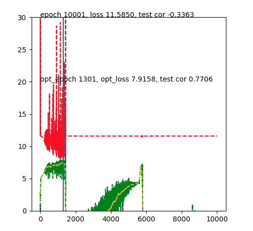
if I run with tune_loss=True (do cv in the fit method with initate_weights before each loop):
net = Model(min_loss = .9, l_rate = 1e-3, max_epochs = 10000)
%matplotlib notebook
net.fit(X_hc, y_hc, tune_loss = True)
I got the curve like this:
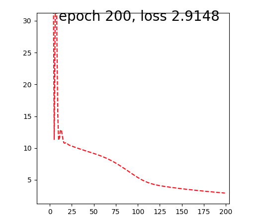
when I run fit in the for loop of 10-fold CV:
for train_index, test_index in kf.split(X):
            print('run_model on CV: %d' % i)

            X_train, X_test = X[train_index], X[test_index]
            y_train, y_test = y[train_index], y[test_index]
            net.fit(X_train, y_train, tune_loss = False)
I got the curve like this:
Could anyone explain why this happens?