Hey, all
I have been trying to understand the PyTorch sine wave example given here: example
It took me some time to digest what actually is happening and how the input/output pair is made in this.
They have used LBFGS and have fed all the batches at once which might not be feasible in every case, thus I was trying to implement the same example using batched way and using Adam Optimizer.
I have also tweaked the Model structure a bit, now my model is like this:
class Sequence(nn.Module):
    def __init__(self):
        super(Sequence, self).__init__()
        self.lstm1 = nn.LSTMCell(1, 50) #only 1 feature in input, 51 is no of features in hidden_state
        self.lstm2 = nn.LSTMCell(50, 50) #prev cell outputs 51, so this input is 51, and it outputs 51 (hidden_dim)
        self.linear = nn.Linear(50, 36) #takes 51 dim to predict 1 value
        self.relu = nn.ReLU()
        self.linear2 = nn.Linear(36, 24)
        self.linear3 = nn.Linear(24, 1)

    def forward(self, input, future = 0):
        outputs = []
        h_t = torch.zeros(input.size(0), 50, dtype = torch.double) #shape is 97x51 (batch,hidden_size)
        c_t = torch.zeros(input.size(0), 50, dtype = torch.double) #shape is 97x51 (batch,hidden_size)
        h_t2 = torch.zeros(input.size(0), 50, dtype = torch.double)
        c_t2 = torch.zeros(input.size(0), 50, dtype = torch.double)

        #hidden state and cell state are set to 0 in every new "batch" of examples

        for input_t in input.split(1, dim = 1): # input_t is of shape [batch_size,1], loop always runs for 999 times
            h_t, c_t = self.lstm1(input_t, (h_t, c_t))
            h_t2, c_t2 = self.lstm2(h_t, (h_t2, c_t2))
            output = self.linear3(self.relu(self.linear2(self.relu(self.linear(h_t2))))) #output is of shape [batch_size, 1], for every time step t, output has (t+1)th value prediction for all sine waves
            outputs += [output]
        for i in range(future):
            h_t, c_t = self.lstm1(output, (h_t, c_t)) #
            h_t2, c_t2 = self.lstm2(h_t, (h_t2, c_t2))
            output = self.linear3(self.relu(self.linear2(self.relu(self.linear(h_t2)))))
            #output = self.linear(h_t2)
            outputs += [output]
        outputs = torch.cat(outputs, dim = 1) #concat predictions across all timesteps from t1 to t999, and future
        return outputs
Optimizer:
optim = torch.optim.Adam(seq.parameters(), lr = 0.08)
Dataset:
class seqDS(Dataset):
    def __init__(self, x, y):
        self.x = x
        self.y = y
        self.len = x.shape[0]
    def __getitem__(self, idx):
        return self.x[idx], self.y[idx]
    def __len__(self):
        return self.len

ds = seqDS(input, target)
Loader:
train_loader = DataLoader(ds, shuffle = False, batch_size = 16)
and finally, the training Loop:
for i in range(50):
    loss = 0.0
    num_len = 0
    seq.train()
    for x,y in train_loader:
        batch_size = x.shape[0]
        y_pred = seq(x)
        optim.zero_grad()
        loss = criterion(y_pred, y)
        loss.backward()
        optim.step()
        num_len += batch_size
        loss += (batch_size * loss.item())
    loss = loss / (num_len)
    print(f"Epoch {i+1}, Loss: {loss}")

    with torch.no_grad():
        future = 1000
        pred = seq(test_input, future=future)
        loss = criterion(pred[:, :-future], test_target)
        print('test loss:', loss.item())
        print("==========================")
        y = pred.detach().numpy()

    plt.figure(figsize=(30,10))
    plt.title('Predict future values for time sequences\n(Dashlines are predicted values)', fontsize=30)
    plt.xlabel('x', fontsize=20)
    plt.ylabel('y', fontsize=20)
    plt.xticks(fontsize=20)
    plt.yticks(fontsize=20)
    def draw(yi, color):
        plt.plot(np.arange(input.size(1)), yi[:input.size(1)], color, linewidth = 2.0)
        plt.plot(np.arange(input.size(1), input.size(1) + future), yi[input.size(1):], color + ':', linewidth = 2.0)
    draw(y[0], 'r')
    draw(y[1], 'g')
    draw(y[2], 'b')
    plt.savefig('predict%d.pdf'%i)
    plt.close()
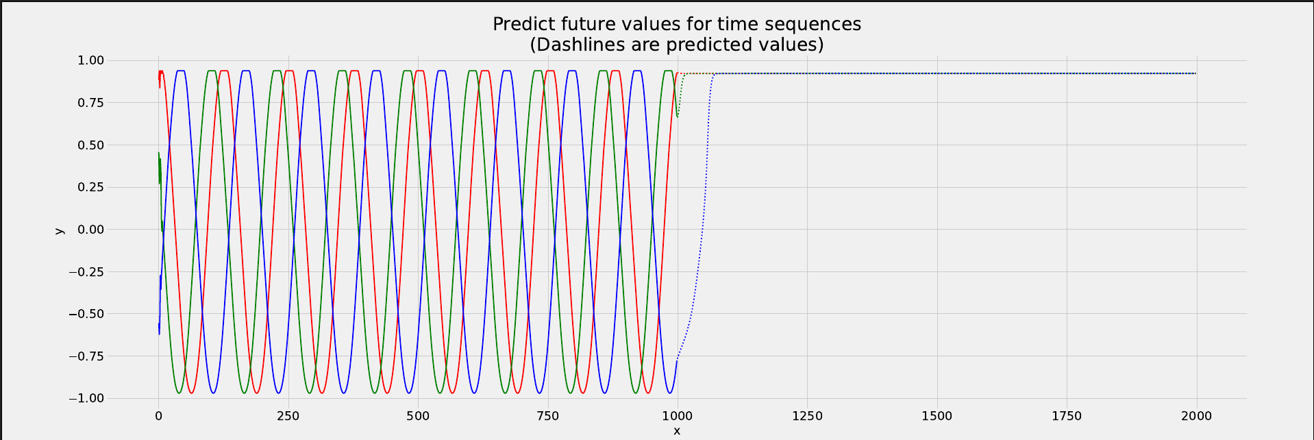
Now, as you can see from this plot below, the results are very disappointing and the model is not able to predict future values properly and even is not very accurate on predicting test set values that have the real ground truth labels.
I really want to go deep into this and understand what is actually happening and how can I fix this, LSTM is supposed to have a memory element due to cell state that’s what I know, and since the cell state used at time t = 0 is propagated to time t = 999, why its still failing to predict the sine wave values for future times (after t = 1000) on the test set data?
Thank you so much for your time.