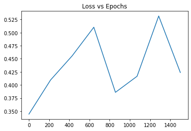
I am messing with my neural network code trying to make it as accurate as possible but I feel like my numbers are not looking right. I have plotted a Loss vs Epoch graph to find out the perfect number of epochs to use for my training loop but that graph doesn’t look right. The loss seems to be spiking every now and then. Loss is on the y-axis and epoch is on the x-axis. Maybe I am graphing it wrong or there is something wrong with my code? Any advice would help!
The graph for 1500 epoch:
Here is an image of my Predictions vs. Actual values with 2000 epoch:
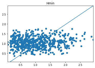
This image is the closest accuracy I could get out of my neural network.
My code:
import torch
import numpy as np
from torch import nn
from torch import optim
from torch.utils.data import TensorDataset
from torch.utils.data import DataLoader
import pandas as pd
import matplotlib.pyplot as plt


'''
Neural Network Structure:
    10 inputs
    10 neurons in the first hidden layer
    2 ouputs
'''

# Get data from tables
# Split data up into training and testing (80% Train, 20% Test)
pnt_cont_data = pd.read_excel('C:\\Users\\bamar\\Downloads\\Chile_Research\\Research_Resources\\DoE_point_contact.xlsm', sheet_name='Sample', index_col = 0, names=['#','E1','E2','v1','v2','Ap','rho0','mue0','u1','u2','R','Fn','hmin','hc','p'])
pnt_cont_data.drop(index = pnt_cont_data.index[0], axis = 0, inplace =True)
del pnt_cont_data['p']

pnt_cont_data = pnt_cont_data.apply(pd.to_numeric, errors='coerce')
pnt_cont_data = pnt_cont_data.dropna()

# Turning data into numpy arrays
X = pnt_cont_data.to_numpy()[:,:-3]
split = int(0.8*len(X))
X_train_np, X_test_np = X[:split], X[split:]

y = pnt_cont_data.to_numpy()[:,11:]

y_train_np, y_test_np = y[:split], y[split:]

y_train_hmin = y_train_np[:,0]
y_train_hc = y_train_np[:,1]

'''
print(X_train_np.shape, y_train_np.shape)
print(X_test_np.shape, y_test_np.shape)

(800, 10) (800, 2)
(200, 10) (200, 2)
'''

X_train_float = X_train_np.astype(np.float32)
X_train = torch.Tensor(X_train_float)


X_test_float = X_test_np.astype(np.float32)
X_test = torch.Tensor(X_test_float)

y_train_float = y_train_np.astype(np.float32)
y_train = torch.Tensor(y_train_float)

y_test_float = y_test_np.astype(np.float32)
y_test = torch.Tensor(y_test_float)

# Creating a train dataset and dataloader with batch_size =50
# Batch size: number of samples processed before the model is updated
train_dataset = TensorDataset(X_train, y_train)
train_dataloader = DataLoader(train_dataset, batch_size = 80)


# Creating a test dataset and dataloader with batch_size = 10
test_dataset = TensorDataset(X_test, y_test)
test_dataloader = DataLoader(test_dataset, batch_size = 10)


########################## Building Neural Network ##########################

device = 'cuda' if torch.cuda.is_available() else 'cpu'

input_dim = 10
hidden_dim = 10
output_dim = 2

class NeuralNetwork(nn.Module):
    def __init__(self, input_dim, hidden_dim, output_dim):
        super(NeuralNetwork, self).__init__()

        # Define and instiante layers
        self.hidden1 = nn.Linear(input_dim,hidden_dim)
        self.hidden_activation = nn.ReLU()
        self.hidden2 = nn.Linear(hidden_dim, input_dim)

        self.out = nn.Linear(hidden_dim, output_dim)

        # Defines what order to inputs will go into each layer
    def forward(self, x):
        y = self.hidden1(x)
        y = self.hidden_activation(x)
        y = self.hidden2(x)
        y = self.hidden_activation(x)

        # no activation function for output of a regression problem
        y = self.out(x)
        return y


# Creating model, putting model in neural network
model = NeuralNetwork(input_dim, hidden_dim, output_dim).to(device)

'''
print(model)

NeuralNetwork(
  (hidden_layer1): Linear(in_features=10, out_features=10, bias=True)
  (hidden_activation): ReLU()
  (out): Linear(in_features=10, out_features=2, bias=True)
)

'''

############################# Training data #############################

# Creating functions for training
# when trying to predict a value, this is a regression problem, therefore MSE is loss function
# learning rate determines a learning STEP
# hyperparameters: what you can control to change the neural network (batch size, learning rate, epoch)
learning_rate = 1.e-6
loss_fn = nn.MSELoss()
# using SGD optimizer
optimizer = torch.optim.SGD(model.parameters(), lr=learning_rate)

# Creating training function
# Iterate over all of our data
def train(dataloader, model, loss_fn, optimizer):
    model.train()
    train_loss_data = []
    train_loss = 0

    # grab index [i] and whatever was in it (X,y)
    for i, (X, y) in enumerate(dataloader):
        X, y = X.to(device), y.to(device)

        # Printing X will print the batch size
        y_pred = model(X)

        # tensor that stores loss function
        loss = loss_fn(y_pred, y)
        train_loss_data.append(loss.item())

        # .item() grabs value of tensor so its just a number
        train_loss += loss.item()


        optimizer.zero_grad()
        loss.backward()
        optimizer.step()
    return train_loss_data

    #print('Total Loss:', train_loss)

        # Calculating RMSE for training
# =============================================================================
#     num_batches = len(dataloader)
#     train_mse = train_loss / num_batches
#
#     # 0.2-0.5 is a good RMSE
#     RMSE = train_mse**(1/2)
#     #print('Train RMSE:', RMSE)
# =============================================================================

def test(dataloader, model, loss_fn):
    model.eval()
    test_loss = 0

    # Turn off back propagation
    with torch.no_grad():
        for X, y in dataloader:
            X, y = X.to(device), y.to(device)

            y_pred = model(X)
            test_loss += loss_fn(y_pred, y).item()

# epoch: one pass over ENTIRE dataset
epochs = 2000

for epoch in range(epochs):
    #print(f'Epoch {epoch+1}:')
    train_loss_data = train(train_dataloader, model, loss_fn, optimizer)


print('Training Complete')
    #test(test_dataloader, model, loss_fn)

epochs_plt = np.linspace(0,2000,len(train_loss_data))


plt.plot(epochs_plt, train_loss_data)
plt.title('Loss vs Epochs')
plt.show()

'''
- Create R^2 graph with predicted vs actual values (subplots)
- Create loss vs epochs graph and choose epoch where its most stable

'''

# Graphing data, evaluating training loop
def Graph_eval(model, X, y):
    model.eval()         # setting model to inference mode

    predictions = []
    pred_hmin = []
    pred_hc = []
    actual_hmin = []
    actual_hc = []

    X, y = X.to(device), y.to(device)

    for i in range(len(X)):
        pred = model(X[i])
        act_hmin = y[i][0]
        act_hc = y[i][1]

        predictions.append(pred.tolist())
        actual_hmin.append(act_hmin.item())
        actual_hc.append(act_hc.item())

    for i in range(len(predictions)):
        predictions_hmin = predictions[i][0]
        predictions_hc = predictions[i][1]

        pred_hmin.append(predictions_hmin)
        pred_hc.append(predictions_hc)

    # Plotting actual vs predictions scatter plot, using subplots
    actual_hmin_min = min(actual_hmin)
    actual_hmin_max = max(actual_hmin)

    actual_hc_min = min(actual_hc)
    actual_hc_max = max(actual_hc)

    plt.scatter(actual_hmin, pred_hmin)
    plt.title('Hmin')
    plt.plot([actual_hc_min, actual_hmin_max], [actual_hmin_min, actual_hmin_max])
    plt.xlim(actual_hmin_min, actual_hmin_max)
    plt.ylim(actual_hmin_min, actual_hmin_max)
# =============================================================================
#     fig, (ax1, ax2) = plt.subplots(1,2)
#     ax1.scatter(actual_hmin, pred_hmin)
#     ax1.set_title('Hmin')
#     ax1.set_xlabel = 'Actual'
#     ax1.set_ylabel = 'Predictions'
#     ax1.plot([actual_hmin_min, actual_hmin_max],[actual_hmin_min, actual_hmin_max])
#
#     ax2.scatter(actual_hc, pred_hc)
#     ax2.set_title('Hc')
#     ax2.set_xlabel = 'Actual'
#
#     ax2.plot([actual_hc_min, actual_hc_max],[actual_hc_min, actual_hc_max])
# =============================================================================
    plt.show()

    return pred_hmin, pred_hc, actual_hmin, actual_hc


pred_hmin, pred_hc, actual_hmin, actual_hc = Graph_eval(model, X_train, y_train)