Manually calculating integrated gradient

in the paper formula is,
Screenshot (485)

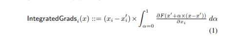
how do we manually calculate this value, for example,

from captum.attr import IntegratedGradients
import torch, torch.nn as nn, torch.nn.functional as F
class ToyModel(nn.Module):
    r"""
    Example toy model from the original paper (page 10)

    https://arxiv.org/pdf/1703.01365.pdf


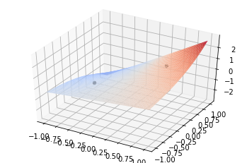
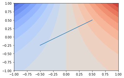
    f(x1, x2) = RELU(ReLU(x1) - 1 - ReLU(x2))
    """

    def __init__(self):
        super().__init__()

    def forward(self, input1, input2):
        relu_out1 = F.relu(input1)
        relu_out2 = F.relu(input2)
        return F.relu(relu_out1 - 1 - relu_out2)
net = ToyModel()
net.eval()
# defining model input tensors
input1 = torch.tensor([3.0], requires_grad=True)
input2 = torch.tensor([1.0], requires_grad=True)

# defining baselines for each input tensor
baseline1 = torch.tensor([0.0])
baseline2 = torch.tensor([0.0])

# defining and applying integrated gradients on ToyModel and the
ig = IntegratedGradients(net)
attributions, approximation_error = ig.attribute((input1, input2),
                                                 baselines=(baseline1, baseline2),
                                                 method='gausslegendre',
                                                 return_convergence_delta=True)
attributions

gives
(tensor([1.5000], grad_fn=),
tensor([-0.5000], grad_fn=))

so, here baseline is 0, 0 input is 3, 1 if our function is,

f(x1, x2) = x1 - 1 - x2

do we replace x1 with x1*alpha, then differentiate wrt x1, so we get alpha, then integrate, so we get alpha**2 / 2 with alpha from 0 to 1, that is 1/2

and same thing for x2, replace x2 with x2*alpha, then differentiate wrt x2, so we get -alpha, then integrate, so we get -alpha**2 / 2 with alpha from 0 to 1, that is -1/2

then multiply these with input, which gives 1.5, -0.5.

what is the intuition behind using this technique, and how does one understand this formula in a better way?

So the goal of the attribution exercise we are doing is to attribute the difference between F(x) and F(x’) to the inidividual components of the input difference (x-x’).
What happens is that we are following the line form x’ to x. If we integrate the derivative in the direction of this line that, we get the difference between F(x) and F(x’), this is the fundamental theorem of calculus.
But now, the “derivative in the direction of this line” can be written as a scalar product of the gradient of F with the direction vector ((x-x’) / |x-x’|). The integrated gradient now collects the gradient of F parts separately (before the scalar product).
This and a change of variables leads to the formula you cite above.
Inherent in the construction is sum_i IntegratedGrads_i(x) = F(x) - F(x’), so we are indeed decomposing the difference.

Best regards

Thomas

I think you explain correct but I am still confused, could you give an example with a function like f(x) = x**2.

A 1d example won’t do. :slight_smile:
But here is a simple 2d one.
Take f(x, y) = x * exp(y). We can plot this in 3d or as a countour plot:

f = lambda x, y: x * y.exp()
xx = torch.linspace(-1,1)[None].expand(100,100)
yy = torch.linspace(-1,1)[:, None].expand(100,100)
zz = f(xx, yy)
x0 = torch.tensor([-0.5, 0.5])
y0 = torch.tensor([-0.25, 0.5])
z0 = f(x0, y0)
fig = pyplot.figure()
ax = fig.gca(projection='3d')
ax.scatter3D(x0[0], y0[0], z0[0], color=['k'], s=20)
ax.scatter3D(x0[1], y0[1], z0[1], color=['k'], s=20)
ax.set_transform
ax.plot_surface(xx.numpy(),yy.numpy(),zz.numpy(), cmap=pyplot.cm.coolwarm)
ax.view_init(elev=40)
pyplot.figure()
pyplot.contourf(xx.numpy(),yy.numpy(),zz.numpy(), cmap=pyplot.cm.coolwarm, levels=20)
pyplot.plot(x0, y0)

3d:

image

Contour plot:
image

Now I added two points (in the 3d) and a line in the countour plot. We take the top right end of the line as x and the lower bottom as x’.

We can parametrize this line:

x_line = (x0[0] + torch.linspace(0, 1, 1000) * (x0[1] - x0[0])).requires_grad_()
y_line = (y0[0] + torch.linspace(0, 1, 1000) * (y0[1] - y0[0])).requires_grad_()

Note that this looks a like the x’ + α(x-x’) you have as an argument to ∂F/∂x_i in the integral in your equation (1).

And indeed we can compute the gradients for each point on the line:

z_line = f(x_line, y_line)
z_line.sum().backward()

We can approximate the integral over 0…1 by taking the mean over the .grads. Thus we can calculate the integrated gradients:

ig_x = (x0[1] - x0[0]) * x_line.grad.mean()
ig_y = (y0[1] - y0[0]) * y_line.grad.mean()

This gives ig_x as 1.1599 and ig_y as 0.0540.

As a sanity check, we can compare ig_x + ig_y with z0[1]-z0[0] and indeed they seem to differ by 0.0001, which looks good.

Best regards

Thomas

4 Likes

thanks for your reply, I carry experiment and find

ig_x + ig_y

and

z0[1] - z0[0]

to be equal to,

1.21376102688577

when integrating, with alpha from 0 to 1.

in the paper, they also have this figure,
Screenshot (489)
does this mean, that instead of parameterization of a line, we could parameterize a curve also, like a sigmoid curve, or a sinusoidal curve, or a circle and that would be a different attribution method.

1 Like

So there are several things to be considered here:

  • The line parametrization (x’ + α(x-x’)) is of constant speed along the path. This enables multiplying with (x_i-x’_i) at the last step rather than having to do this separately for each “time step” in the integral. But done properly such a change of in the parametrization of the path would not change the result.
  • As the figure illustrates, if you took a path different than the straight line, then you would get a different attribution. While the “sum of the two attribution parts” is again the difference in function values by the fundamental theorem of calculus, you can get a wildly different split by coordinate. e.g. if you take F = min(x_1, x_2) as your function and consider paths between (0, 1) and (1, 0), where the function is both 0. You could go along the coordinate axes to get (depending on which you do first) an attribution of (0, 0) or (1, -1). You can also get anything in between by interleaving directions.
  • One of the bad parts of all this (with having to arbitrarily choose the line) is that it will no compose well, i.e. if you declare the last conv layer of your network the features and now you want to attribute the change in features to the change in input and the change in output to the change in features, you’ll get something completely different between the two, because it’s unlikely that the straight line in input space corresponds to a straight line in feature-space.
  • In the end, it is some sort of non-definedness issue around the choice of path. The next question could be how to get around this. The straight line is straightforward to pick in Euclidean space, as would be geodesics (but even then it might not be unique if you have several) for manifolds. You could also try to get avoid the choice of a single path by introducing some probability measure on the paths and then integrating over that. But by then you’re in a much more complex setting (and I’m not sure anyone has done this).

Hmhm. Now the last post might have been peak happiness. :slight_smile:

Best regards

Thomas