Medical binary classification with BCE Loss: threshold?

Hello everyone!
I am a med resident that really enjoy learning about ML, I spent a lot of time reading here and want to make use of it in my field, medical imaging. We have an exam called “Datscan scintigraphy” which is a metabolic view of people’s brain to see if they have Parkinson disease or not (it’s a simplification but enough to understand).

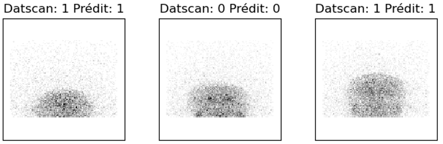
The problem is that it’s a long exam that takes about 30 min because the “camera” turns around the patient 120 times. So sometimes, our elder patient can’t stand it and it’s frustrating to not be able to help them with a diagnosis. This is why I’m building a CNN trying to classify between “Normal Datscan” or “Abnormal Datscan” with only the first 2 projections (anterior and posterior, number 0 and 60), with as a final output a “probability of abnormal datscan” between 0 and 1.
My goal is that after I get this probability, I could change the threshold and make it more sensitive or more specific, according to what we want.

I built a dataset with 887 datscans converted as npy arrays of each 120 of 128x128 pixel matrix, and only use 2 of them (number 0 and 60). It’s grayscale images so 1 in channel.
I tried different architectures, here is the VGG one with BCEWithLogitsLoss:

class ReseauConvolutionSigmo(nn.Module):
def __init__(self):
    super(ReseauConvolutionSigmo, self).__init__()
    self.conv1a = nn.Conv2d(2, 64, 3, stride=1)
    self.conv1b = nn.Conv2d(64, 64, 5, stride=1)
    self.pool1 = nn.MaxPool2d(2,2)

    self.conv2a = nn.Conv2d(64, 128, 3, stride=1)
    self.conv2b = nn.Conv2d(128, 128, 3, stride=1)
    self.pool2 = nn.MaxPool2d(2,2)
    
    self.conv3a = nn.Conv2d(128, 256, 3, stride=1)
    self.conv3b = nn.Conv2d(256, 256, 3, stride=1)
    self.pool3 = nn.MaxPool2d(2,2)
            
    self.fc1 = nn.Linear(36864, 84)  
    self.fc2 = nn.Linear(84, 1)       
    
def forward(self, x):
    x=x.float()
    
    x=self.conv1a(x)
    x=F.relu(x)
    x=self.conv1b(x)
    x=F.relu(x)
    x=self.pool1(x)
    
    x=self.conv2a(x)
    x=F.relu(x)
    x=self.conv2b(x)
    x=F.relu(x)
    x=self.pool2(x)
    
    x=self.conv3a(x)
    x=F.relu(x)
    x=self.conv3b(x)
    x=F.relu(x)
    x=self.pool3(x)
    
    x = torch.flatten(x, 1)  # Flatten the feature maps
    
    try:
        x = F.relu(self.fc1(x))
    except RuntimeError as e:
        e = str(e)
        if e.endswith("Output size is too small"):
            print("Image size is too small.")
        elif "shapes cannot be multiplied" in e:
            required_shape = e[e.index("x") + 1:].split(" ")[0]
            print(f"Linear layer needs to have size: {required_shape}")
        else:
            print(f"Error other: {e}") 
            
    x = self.fc2(x)

    return x
n_epochs = 100
criterion = nn.BCEWithLogitsLoss()
optimizer = optim.Adam(network.parameters(), lr=0.001)

train_losses = [ ]
train_counter = [ ]
test_losses = [ ]
test_accuracy = [ ]

network.to(device)
print('******* Evaluation initiale')
test()
for epoch in range(0, n_epochs):
  print('******* Epoch ',epoch)
  train()
  test()

But when doing so, the output tensors of the 6 elements of the batch all quickly converge to the same value,

Summary
******* Evaluation initiale
test loss= 0.7000894740570424
Output tensor([[0.0826],
        [0.0827],
        [0.0827],
        [0.0825],
        [0.0827],
        [0.0827]])
Predicted tensor([[0.], [0.], [0.],[0.],[0.], [0.]])
Datscan tensor([[0.],[0.], [0.],[1.],[0.],[1.]])
Accuracy in test 57.36434108527132 %
******* Epoch  0
train loss= 0.6777993538058721
test loss= 0.6830593472303346
Output tensor([[-0.3489],
        [-0.3479],
        [-0.3391],
        [-0.3410],
        [-0.3442],
        [-0.3469]])
Predicted tensor([[0.], [0.], [0.],[0.],[0.], [0.]])
Datscan tensor([[1.], [0.],[0.],[0.], [0.],[0.]])
Accuracy in test 57.36434108527132 %
******* Epoch  1
train loss= 0.7050089922088844
test loss= 0.6875958317934081
Output tensor([[-0.0826],
        [-0.0826],
        [-0.0826],
        [-0.0826],
        [-0.0826],
        [-0.0826]])
Predicted tensor([[0.], [0.], [0.],[0.],[0.], [0.]])
Datscan tensor([[0.], [0.],[1.],[1.], [0.], [1.]])
Accuracy in test 57.751937984496124 %
******* Epoch  2
train loss= 0.6914097838676893
test loss= 0.6917881480483121
Output tensor([[-0.0191],
        [-0.0191],
        [-0.0191],
        [-0.0191],
        [-0.0191],
        [-0.0191]])
Predicted tensor([[0.], [0.], [0.],[0.],[0.], [0.]])
Datscan tensor([[0.],[1.], [1.],[1.],[0.],[1.]])
Accuracy in test 57.36434108527132 %

#### Even at late epoch:
******* Epoch  40
train loss= 0.6704580792440817
test loss= 0.6978785312452982
Output tensor([[-0.6284],
        [-0.6284],
        [-0.6284],
        [-0.6284],
        [-0.6284],
        [-0.6284]])
Predicted tensor([[0.], [0.], [0.],[0.],[0.], [0.]])
Datscan tensor([[0.],[0.], [0.],[0.],[1.],[1.]])
correct 147
total 258
Accuracy in test 56.97674418604651 %

So as you can see, the training loss doesn’t decrease that much, and the accuracy is stuck at 57%.

I was kinda desesperate and tried with another criterion: CrossEntropy:
There it worked really better, with a final accuracy of 79% here for example the 3 last epochs:

Summary
******* Epoch  47
train loss= 0.0002839015607657339
test loss= 1.7087745488627646
correct 203
total 258
Accuracy in test 78.68217054263566 %
Sortie du réseau :
tensor([[-13.9290,   4.8103],
        [  3.7896,  -9.5477],
        [ -3.8057,  -0.1662],
        [  1.8018,  -3.5083],
        [ -3.6199,  -2.2624],
        [  6.0148, -12.3137]])
Datscan :    tensor([1, 1, 0, 0, 1, 0])
Prédiction :  tensor([1, 0, 1, 0, 1, 0])
 
******* Epoch  48
train loss= 0.0002534455537248284
test loss= 1.7621866015008938
correct 201
total 258
Accuracy in test 77.90697674418605 %
Sortie du réseau :
tensor([[-24.7145,   7.8902],
        [-21.3964,   8.6213],
        [  2.1064,  -0.7032],
        [ -1.3331,  -0.8390],
        [ -5.9108,   4.1722],
        [-14.4751,   4.5746]])
Datscan :    tensor([1, 1, 0, 1, 1, 1])
Prédiction :  tensor([1, 1, 0, 1, 1, 1])
 
******* Epoch  49
train loss= 0.00022697989463199136
test loss= 1.6694575882692397
correct 204
total 258
Accuracy in test 79.06976744186046 %
Sortie du réseau :
tensor([[ -9.4081,   1.5622],
        [ -0.1025,   0.0649],
        [-26.1112,   8.3820],
        [-12.4035,   3.2135],
        [ -6.0753,   0.1667],
        [  9.9138,  -9.7220]])
Datscan :    tensor([0, 0, 1, 1, 1, 0])
Prédiction :  tensor([1, 1, 1, 1, 1, 0])
 
 
Sortie du réseau :
tensor([[ 14.8245, -11.1206],
        [  4.8293,  -2.1229],
        [-19.1812,   4.6617],
        [ -7.9391,   3.3256],
        [ 30.0683, -26.7278],
        [-11.0685,   3.2678]])
 
Datscan :    tensor([0, 1, 1, 1, 0, 1])
Prédiction :  tensor([0, 0, 1, 1, 0, 1])

So here are my questions:

  • What makes the BCEloss train so badly even if it is a binary classification problem? And how come all the 6 element of the batch end up quickly toward the same output tensor?
    I tried changing the learning rate but without a clear improvement, maybe it’s the optimizer?

  • From my understanding, the output in the BCEWithLogitsLoss are the 6 tensors of the batch, and he predicts “normal” if the output tensor is negative and “abnormal” if positive. But they’re stuck in negative so they’re all predicted normal.
    Since my goal is to make a “probability of abnormal datscan output” , if this model had a better accuracy I could just use this output tensor in a sigmoid and create a 0 to 1 probability right?

  • The output in the CrossEntropyLoss version are 2 x 6 Tensors, representing the “confidence” in being in the left class (so “normal”) or the right class (so “abnormal”), and the higher tensor value is the predicted class. For example:
    tensor([[ 14.8245, -11.1206], = predicted normal
    [ 4.8293, -2.1229], = predicted normal
    [-19.1812, 4.6617], = predicted abnormal
    [ -7.9391, 3.3256], = predicted abnormal
    [ 30.0683, -26.7278], = predicted normal
    [-11.0685, 3.2678]]) = predicted abnormal

However, while it has a better accuracy, the problem is how can I represent these output tensors as “probability of being abnormal”?

Thank you very much for your help, and I look forward to reading your thoughts about it, it’s always extremely interesting!

Hi Quazality!

There’s a lot going on here … Let me start with some preliminary questions.

Am I correct that this result is from before any optimization steps have
been taken?

As I read this, the output (for one of your test batches) is a batch of six
logits, each of which corresponds to the probability of the associated
sample in the input batch being “abnormal,” as they are all positive. Is
this correct? But then your “Predicted tensor” is all 0.s, which I would
have thought meant “normal.”

As you noted, the outputs for each of the samples in you batch are the
same (to three decimal digits). This seems quite odd.

I assume that this again is for a single test batch, but now after having
taking one epoch’s worth of optimization steps. Correct?

Now your six predicted logits are all quite close (but only agree to about
two decimal digits) and are all negative (= “normal”?). But your “Predicted
tensor” is still all 0.s. So how do you convert from your “Output tensor”
to your “Predicted tensor?” Something just doesn’t look right here.

Am I correct that the input to your model is a tensor with shape
[6, 2, 128, 128], where 6 is the number of samples in a given batch,
2 is the number of channels (one being the anterior and the other being
the posterior projection*), and the 128, 128 is the height and width of the
image in pixels?

What do the input images look like? Do they look more or less like random
noise? If I looked at one, would I say there’s a skull with a brain inside?
If you looked at an image, with your expertise, would you be able to tell
with reasonable accuracy whether it represented a “Normal Datascan”
vs. an “Abnormal Datascan?”

What values do your pixels range over? Do you perform any sort of
normalization? I see x=x.float() inside of your model’s forward()
function. What is the dtype of the tensor you input to your model?

Do I assume correctly that when you did this the only change you made
to your model was changing the final fc2 layer from nn.Linear (84, 1)
to nn.Linear (84, 2)?

What does your CrossEntropyLoss-version output look like before you
perform any optimization steps, that is, its “Evaluation initiale” output?

The reason I ask is that output of your BCEWithLogitsLoss-version is
rather small in magnitude – on the order of 0.1, while the magnitude of
your CrossEntropyLoss output (after training) is significantly larger – on
the order of 10.0.

Just to be clear, you are using BCEWithLogitsLoss. Correct? Also, just
to confirm, you are not passing the output of your model through any sort
of sigmoid() before you pass it to the loss function. Is this also correct?

It looks like this version of your training is broken somehow. In general,
your two versions – BCEWithLogitsLoss with one model output and
CrossEntropyLoss with two outputs – should behave quite similarly, so
this difference is surprising. Double check for any bugs that might have
slipped in.

This also strikes me as odd, which is why seeing the CrossEntropyLoss
output before any training could be informative.

Adam often trains faster, but can behave oddly at times. I would suggest
trying plain-vanilla SGD with a small learning rate. After you see how things
look, you could try turning up the learning rate and turning on momentum
as long as your training appears to stay stable.

Except that the first result you posted was positive for all six samples in
the batch (even though you had 0.s in your “Predicted tensor”).

If I understand you correctly, yes. probability = sigmoid (logit).

Yes.

For a multi-class problem (in your case two-class) the output of a
model trained with CrossEntropyLoss will be a set of unnormalized
log-probabilities for each of your classes.

Let’s say you had six classes – you would predict six unnormalized
log-probabilities. But you only have five degrees of freedom as the
final (normalized) probabilities must add up to one. To convert the
output of your model to (normalized) probabilities, pass it though
softmax() (the output of which will sum to one).

Consider:

>>> output = torch.tensor ([[-3.8057,  -0.1662]])
>>> probs = output.softmax (-1)
>>> probs
tensor([[0.0256, 0.9744]])
>>> probs.sum()
tensor(1.)

As you say, the class with the algebraically larger output value is the
class you are predicting. softmax (output) then gives you the predicted
probabilities (which sum to one). So in the above example, you are
predicting “Abnormal” with a probability of 97.4%, that is to say with
near certainty.

Note that the only thing that matters is the difference between the
predicted unnormalized log-probabilities for the two classes. (This is
a reflection of the fact that there is only one degree of freedom.)

Consider:

>>> output2 = output + 1.234
>>> output2
tensor([[-2.5717,  1.0678]])
>>> output2.softmax (-1)
tensor([[0.0256, 0.9744]])

*) As an aside, I imagine that the anterior projection (channel 0 of your
input tensor) would show the right half of the patient’s brain on the left
side of the image, while the posterior projection (channel 1) would show
the right half of the patient’s brain on the right side of the image (or maybe
vice versa).

If this is the case, it might make it easier for your model if you were to flip
channel 1 of your input images left-for-right so that the initial two-channel
convolution of your model will be combining information from the same
part of the brain in its initial processing.

Best.

K. Frank

1 Like

Thanks a lot for your answer,! I followed a lot of your posts in this forum and I am honored that you took the time to detail such a reply
I will add all the elements you asked:

  • First, I will share with you the train and test functions:
    The one I use for BCEWithLogitsLoss:
def train():
  network.train()
  train_loss=0
  for batch_idx, (datscan,projections) in enumerate(train_loader):

    datscan,projections  = datscan.to(device), projections.to(device)
    datscan = datscan.unsqueeze(1).float()
    optimizer.zero_grad()
    output = network(projections)
    loss = criterion(output, datscan)
    loss.backward()
    optimizer.step()
    train_loss += loss.item()
    
  train_loss=train_loss/len(train_loader)
  print("train loss=",train_loss)  
  train_losses.append(train_loss)

def test():
  network.eval()
  test_loss = 0
  correct = 0
  total = 0
  with torch.no_grad():
    for batch_idx, (datscan,projections) in enumerate(test_loader):
      datscan,projections  = datscan.to(device), projections.to(device)
      datscan = datscan.unsqueeze(1).float()
      output = network(projections)
      loss = criterion(output, datscan)
      predicted = (output > 0).float()
      total += datscan.size(0)
      correct += (predicted == datscan).sum().item()
      test_loss += loss.item()
        
  test_loss=test_loss/len(test_loader)  
  print("test loss=",test_loss) 
  test_losses.append(test_loss)
  print('Output', output)
  print('Predicted', predicted)
  print('Datscan', datscan)
  print('Accuracy in test', (100.0 * correct / total),'%')
  test_accuracy.append((100.0 * correct / total))

Maybe the line predicted = (output > 0).float() isn’t correct?

  • And the training/testing functions for the CrossEntropyLoss criterion version are exactly the same, except the line predicted = (output > 0).float() , which is changed by: _, predicted = torch.max(output.data, 1), since it returns the index of the highest output tensor of each pair (so 0 if normal, 1 if abnormal)

Am I correct that this result is from before any optimization steps have
been taken?

Exactly!

Oh you’re right, the predicted tensor being all 0 while the Output numbers are positive isn’t logical! It must have been because in the first versions I wrote predicted = (output > 0,5).float() but I changed it, so now it displays 1 when positive and 0 when negative.

However the outputs for each of the samples are still quickly becoming the same, hmmm

Exactly. The input images kinda look like a pixelized view of a brain, one from the front and one from the back


Here I printed the front one of three samples (number 0)

If it was me with my expertise, with the 120 projections I could classify them, but with only the 2 (anterior and posterior) I would say I have a pretty limited accuracy, close of the 80% of the VGG CrossEntropyLoss one.

The pixel values are from 0 to 30 for each projection (the 120 128x128 matrix), it represents the number of photons the detector of this pixel caught during the 30s recording of this angle. But when I created the npy.array representing each projection of each patient, I normalized it by dividing with the maximum value /np.max(study.pixel_array[projection_number,:,:]))

I checked and apparently, in the train and test function, the tensor I input in the model are:

datscan,projections = datscan.to(device), projections.to(device)
“datscan” is a torch.int64, “projections” is a torch.float64

datscan = datscan.unsqueeze(1).float()
“datscan” is a torch.float32

optimizer.zero_grad()
output = network(projections)
loss = criterion(output, datscan)

Indeed, that’s the only change in the model, though I also adjusted the train and test function as I showed you in the begining.

Here:

******* Evaluation initiale
test loss= 0.6907461174698764
Accuracy in test 57.36434108527132 %
Sortie du réseau :
tensor([[ 0.0300, -0.0047],
        [ 0.0300, -0.0047],
        [ 0.0301, -0.0047],
        [ 0.0299, -0.0048],
        [ 0.0300, -0.0047],
        [ 0.0300, -0.0048]])
Datscan :    tensor([1, 1, 1, 0, 1, 1])
Prédiction :  tensor([0, 0, 0, 0, 0, 0])

As you can see, it starts rather small too, and the output tensors are really similar for all the 6 samples of the batch. However, you see a classification improvement from the 11th epoch:

Epoch 10, 11 and 12
******* Epoch  10
train loss= 0.6694040123659831
test loss= 0.6816538738649945
Accuracy in test 57.751937984496124 %
Sortie du réseau :
tensor([[ 0.3853, -0.1837],
        [ 0.3339, -0.1281],
        [ 0.3601, -0.1145],
        [ 0.3801, -0.1593],
        [ 0.3785, -0.1978],
        [ 0.3705, -0.1680]])
Datscan :    tensor([0, 1, 0, 0, 0, 1])
Prédiction :  tensor([0, 0, 0, 0, 0, 0])
 
******* Epoch  11
train loss= 0.640837006844007
test loss= 0.6732482120048168
Accuracy in test 59.30232558139535 %
Sortie du réseau :
tensor([[-0.2082,  0.0615],
        [-0.1359,  0.0282],
        [-0.0950, -0.0272],
        [ 0.0529, -0.1917],
        [-0.2526,  0.1207],
        [-0.1746,  0.0579]])
Datscan :    tensor([0, 0, 1, 0, 1, 0])
Prédiction :  tensor([1, 1, 1, 0, 1, 1])
 
******* Epoch  12
train loss= 0.6197030756335992
test loss= 0.6258847131285556
Accuracy in test 60.46511627906977 %
Sortie du réseau :
tensor([[ 0.6770, -0.9452],
        [ 0.1119, -0.2286],
        [-0.0486, -0.2046],
        [-0.2933, -0.0825],
        [ 0.1650, -0.4114],
        [ 0.3561, -0.3583]])
Datscan :    tensor([0, 1, 1, 1, 1, 1])
Prédiction :  tensor([0, 0, 0, 1, 0, 0])
 
******* Epoch  13
train loss= 0.5488332117406222
test loss= 0.5568175250014593
Accuracy in test 68.6046511627907 %
Sortie du réseau :
tensor([[ 0.0979, -0.9573],
        [ 0.8947, -1.7356],
        [ 0.8428, -1.8251],
        [ 0.9396, -2.2255],
        [ 0.5075, -1.4734],
        [-0.0085, -0.9892]])
Datscan :    tensor([1, 0, 0, 0, 0, 0])

Correct, I read your replies in other posts and made sure to let BCEWithLogitsLoss without adding any sigmoid.

And indeed, if it is supposed to behave the same, the bug is probably from the “predicted” value I must have failed in the BCEWithLogitsLoss version…

Thank you very much for the softmax clear example, I will try it!
And the aside comment is brilliant too ahah, I have to try the flip. (Btw at first I wanted to use the geometric mean of the 2 projections to insert just one matrix in the first convolution layer, but your idea is way more elegant)

Honestly I can’t thank you enough K Frank, and I hope I answered all your preliminary questions

Hi Quazality!

From a practical point of view, your two-output, CrossEntropyLoss
training seems to be producing a working model, so you could just
go with that.

However …

I don’t see anything wrong with the code you posted (Not that there
isn’t a bug somewhere – I just don’t happen to see one.), so you
really ought to be able to get the one-output, BCEWithLogitsLoss
version working too.

(In practice, I don’t think it really matters which version you use. I
would expect both versions to perform essentially equally well. For
non-compelling reasons, I would expect the one-output version to
be marginally more efficient, but not enough to really matter.)

Here’s what I guess is going on with your one-output version: For
whatever reason, it starts out training slowly, and never really gets
going, even after forty epochs. Try training with a significantly larger
learning rate. (If the training is unstable or starts to diverge, tune
your learning rate down, but try to keep it rather larger than the 0.001
you reported using.)

If training does start to make progress, my bet is that you could then
lower the learning rate back down to 0.001 – not that you would
necessarily want to – and still have training progress.

Please also try plain-vanilla SGD, potentially with a rather large learning
rate, say, perhaps, 0.1. Back off if training is unstable. Again, I bet if
you can get training to progress, it will keep progressing, even if you
lower the learning rate – again, not that you would necessarily want to.

Last, not that you would necessarily want to perform this experiment, you
could pre-train all of your model using two-output training (since this training
does progress), replace fc2 with a new, randomly-initialized single-output
version, and then continue training this single-output version (using
BCEWithLogitsLoss as the loss criterion). The idea would be that the
two-output training gets the network “unstuck” from its randomly-initialized
starting point, after which single-output training would progress reasonably
well.

Additional comments in line, below:

This is fine – this is probably the cleanest way to compute predicted.
(Also, this is only for your accuracy, so it doesn’t affect the training issue.)

I would say that the outputs are starting out being the same.

Could you print out fc2.bias, as well as output (for a couple of batches)
before performing any optimization steps?

My working hypothesis is that between the random initialization of the
preceding layers and the noisy character of the input images, the input
to fc2 has been averaged down close to zero, so that the output of
fc2 is essentially just its .bias. If this is the case, then until the network
has started to train away from its initial random state, the upstream
parameters are, in a sense, “disconnected” from the output, so the initial
training stages make very little progress.

(Please print out fc2.bias and a couple of batches of outputs for your
two-output version, as well. I expect that the same thing is happening
there, just not as dramatically as in the one-output case.)

Yes, this is consistent with the notion that more-or-less the same thing is
happening with the two-output version as with the one-output version.

This looks like after ten epochs the two-output training is still rather “stuck,”
but starts to progress more reasonably over the next few epochs.

This is consistent with the notion that both the one-output and two-output
versions are being affected by slow initial training, but with the two-output
version not being affected as badly.

(I’ve seen this behavior in some experiments with unrealistically small
toy models where I’ve compared one-output and two-output training.
After tuning the learning rate (and momentum, if I was using it), both
versions performed about the same, but for “generic,” untuned values
of the learning rate, the two-output version trained faster. It wasn’t clear
to me whether this was enough to say that the two-output version was
“better,” because with minor tuning of the learning rate – which you would
do in any event – the two-output version wasn’t really better, but is was
as if the two-output version were more “resilient” to having its learning
rate away from its optimum value. I wonder if you are seeing the same
kind of thing here.)

Just to confirm what I said above, it looks like you are computing the
“predicted” value correctly (and, regardless, it doesn’t affect the training).

To summarize (barring some bug somewhere that I don’t see), I think
that both your one-output and two-output versions are suffering from
“slow initial training” due to the random initialization of the model layers,
possibly exacerbated by the “noisiness” of your input images.

I bet that you can get your one-output version to train successfully, either
by training (much?) longer or using a larger learning rate (maybe with SGD)
or using some other scheme to jostle it out of its “stuck” initial training.

But, again, your two-output version seems to be working, so there’s not
necessarily any practical reason to spend time sorting out what’s going
on with your one-output version.

Good luck!

K. Frank

1 Like