Roughly I understand that retain_graph will restore the memory which should have been released after calling backward().
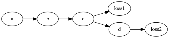
I just wonder, if I have a multi-task computational graph as below, what’s the difference between (loss1+loss2).backward()
and loss1.backward(retain_graph=True); loss2.backward()?
since you have not done a zero_grad operation after loss1.backward(..), they will have the same impact. You can see the gradients or do a step to verify this. Doing the 2 steps separately allows you to inspect the gradients of individual losses, but may cause confusion as they involve an implicit accumulation of gradients ( because you are not doing zero_grad between taking the gradients of the 2 losses)
Joint backward and “piecewise” backward is the usually the same because the joint bits of the graph a) have the same input and b) are all linear in the gradient by the chain rule.
In @zeakey’s d(loss1)/db = dc/db * d(loss1)/dc ; d(loss2)/db = db/dc * d(loss2)/dc, because db/dc is the same, so you can add up the second factor.
Now if you do things in your backward that don’t follow the chain rule - e.g. Graves’-style gradient clipping during the backward - you might have different results between the two. Similarly, when you run into floats are not mathematicians’ real numbers things (NaN, infty, numerical precision), you will see differences.
The main reason to do things separately is probably memory limitations.
A similar insight - except that you split by batches and have (more or less - see batch norm) independent forwards - also powers data parallel.
Thanks for you guys @tumble-weed@tom for helpful insights.
So now I understand that for most common cases the joint backward may be more elegant solution and
they performs identically.