I have seen some triplet loss implementations in PyTorch, which call model.forward on anchor, positive and negative images; then compute triplet loss and finally call loss.backward and optimizer.step, something like this:
I think these implementations are not correct, since it will only consider the outputs of neg_embed = model.forward(neg_images) during bakpropagation, and disregard the anchor and positive images. As far as I know, in PyTorch, gradients are accumulated, but when we call model.forward it will overwrite the previous computations (which makes sense).
Then, the right implementation should concatenate the anchor,positive,negative images and perform a single model.forward, then compute loss and finally loss.backward and optimizer.step.
When you compute the forward pass using different inputs, each output will have its own computation graph attached to it. It’s not overwritten by the next call, so there should be no problem in your current approach.
You are right that the gradients are accumulated in consecutive backward calls, but that doesn’t seem to be the case in your example.
Thanks.
So, this means, three computation graphs will be computed in my example, one for each forward pass.
Then, when we do loss.backward, the gradients will be computed for each computation graph using the same loss.
Finally, the optimizer will update the weights using all three graphs.
Then, the question is, would this be equivalent to doing a single forward pass on the concatenated inputs and then doing loss.backward (which is the intended outcome)?
Even if they are mathematically equivalent (? need to check), the three computation graphs make it inefficient.
Were you able to ever verify this?
For my experiment the 2 are coming out to be not equivalent. Multiple forward passes tho slower and memory inefficient is leading to better score and I’m not at all sure why.
In my experiments, the results were similar. There might be slight differences though. The difference in your case might be due to batch size: the effective batch size might be larger in multiple forward passes.
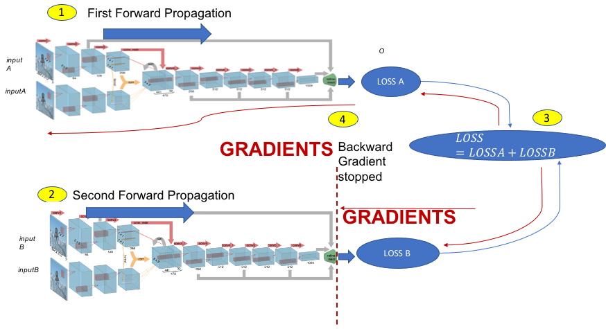
I am in a similar situation. In the pseudo code below I try to do some multiple forward pass before computing the loss.
when grad == no. there is no gradient flowing in the second forward pass (see picture)
when grad == yes the gradient is let flow through the second dynamic graph.
I have observed differences in these two cases.
I went through many posts and cannot understand what is going on under the hood.
To my understanding when doing forward pass with gradient. 2 values per node(of the dynamic graph) are created. We have 2 backward graphs, but linked to the same model, thus
1- How are the weights updated these cases?
2- Same question as @blackberry: are these approaches equivalent to doing a single forward pass on the concatenated inputs and then doing loss.backward ?
My understanding is that they are NOT always equivalent, but close. For example, if there are batchnorm layers in the network, the batchnorm parameters will be updated differently due to different batch sizes.
There might be other (behind the scenes) differences too.
So, if you have memory, it is probably better to do a single forward pass.
I see, we are “artificially changing the batch size” when doing multiple forward propagations.
I understand it would be better to stick to known behaviors, but I find it interesting to do multiple forward propagations because it allows for more flexibility of the network.
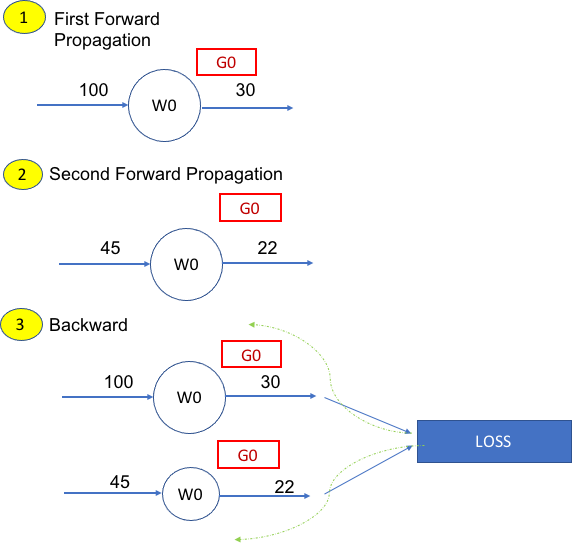
So referring to case args.GRAD == True of my previous example. And referring to the figure below representing one single learnable weight W0. How will W0 be updated after the backpropagation?
Steps.
1 forward propagate inputs (will create G0 to populate the gradient)
2 forward propagate other inputs (will create G0 to populate the gradient), creates new dynamic graph linked to the same network and rooted at LOSS
3 Calculate backward (green dashed arrows). Now we have two gradient values assigned to the same weight
4 How is W0 Updated? What’s the mechanism?
Could you give me some more hints? Maybe a toy example to figure out what is going on? @ptrblck@albanD@blackberry
The two W0 there are actually a single Tensor that is used twice.
So just like any other case where you re-use a Tensor, the mathematical result is to accumulate the contributions for each use of it.
If you use something like torchviz (https://github.com/szagoruyko/pytorchviz/) to print the computational graph, you will see that both evaluations point to a single circle for each weights.