Hi,
Thanks for the response and sorry for the very long response, I hope that the problem will become clearer.
I shall also add that members of the group that I am currently working in with are creating distribution classes in PyTorch and we are more than happy to contribute to developing a scipy.stats style package in PyTorch, as it will not only be useful to us, but I imagine a lot of others too .
So for example, take a simple conjugate Gaussian model:
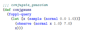
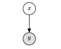
Where the latent variable is x and the observed value is y.
When the above code is translated into python code, we get something like this:
*note VariableCast is just a function that we wrote that converts scalars, numpy arrays and tensors to Pytorch variables, with requires_grad= False. BaseClass is what all ‘programs’ (a graphical model) inherit, that contains a method called calc_grad(output, input), which basically just calls torch.autograd.grad(output=‘log of the joint of the graphical model’, input = ‘latent parameters’) and returns the gradients of the log joint w.r.t latent parameters:
class conjgauss(BaseProgram):
         def __init__(self):
         super().__init__()

  def generate(self):
     ''' Generates the initial state and returns the samples and logjoint
         Only called at the start of the HMC Loop '''

     ################## Start FOPPL input ##########
     logp = [] # empty list to store logp's of each latent parameter
     dim = 1
     params = Variable(torch.FloatTensor(1,dim).zero_())
     mean1 = VariableCast(0.0)
     std1 = VariableCast(2.236)
     normal_object = Normal(mean1, std1)
     x = Variable(normal_object.sample().data, requires_grad = True)
     params = x

     std2    = VariableCast(1.4142)
     y       = VariableCast(7.0)
     p_y_g_x    = Normal(params[0,:], std2)

     ################# End FOPPL output ############
     dim_values = params.size()[0]
     logp.append(normal_object.logpdf(params))
     logp.append(p_y_g_x.logpdf(y))

     # sum up all log probabilities
     logp_x_y   = VariableCast(torch.zeros(1,1))
     for logprob in logp:
         logp_x_y = logp_x_y + logprob
     return logp_x_y, params, VariableCast(self.calc_grad(logp_x_y,params)), dim_values

def eval(self, values, grad= False, grad_loop= False):
     '''This will be continually called within the leapfrog step
     '''
    logp = []  # empty list to store logp's of each latent parameter
    assert (isinstance(values, Variable))
    ################## Start FOPPL input ##########
    values = Variable(values.data, requires_grad = True) # This is our new 'x'
    mean1 = VariableCast(0.0)
    std1 = VariableCast(2.236)
    normal_object = Normal(mean1, std1)

    std2 = VariableCast(1.4142)
    y      = VariableCast(7.0)
    p_y_g_x    = Normal(values[0,:], std2)

    logp.append(normal_object.logpdf(values[0,:]))
    logp.append(p_y_g_x.logpdf(y))

    ################# End FOPPL output ############
    logjoint = VariableCast(torch.zeros(1, 1))

    for logprob in logp:
        logjoint = logjoint + logprob
    if grad:
        gradients = self.calc_grad(logjoint, values)
        return gradients
    elif grad_loop:
        gradients = self.calc_grad(logjoint, values)
        return logjoint, gradients
    else:
        return logjoint, values
So when I mean the graph, on the one hand, I mean the computation graph that Pytorch constructs between Start FOPPL input and End FOPPL output and the graph that it is physically modelling, given by the simple directed graph above. Because the conjgauss.eval() method is called at every interation bar the the first, the only thing that has changed is x is now replaced by values, which are generated during a step within the HMC algorithm. So, the directed graph structure remains fixed and all that is changing in the Pytorch graph and the directed graph, is the values in the conjgauss.eval() method. But because of the way I have implemented it, the whole graph is created at each iteration, which could be called, for example, 18000 times if running the algorithm to generate 1000 samples. So is there a way to retain the Pytorch graph structure and just update the latent parameters, values, within that graph. And then just call torch.autograd.grad() on the newly updated graph.