PyTorch training issue with EfficientNetB3 | Validation Accuracy plateu

[Marco]

Before I start, I wanted to add that I’m relatively new to deep learning, so my setup may be overly complex or suboptimal.

I’m training an image classification model (EfficientNet-B3 on grayscale Kanji images) using PyTorch with:

• AMP (torch.amp.autocast + GradScaler)

• class-balanced split dataset from HDF5

• Input: (1, 128, 128) grayscale images (~620000 images across 3036 classes)

• Loss: CrossEntropyLoss (label smoothing = 0.1)

• Optimizer: AdamW (weight decay = 1e-4)

During training, I observe that my validation accuracy keeps plateauing around 65%.

My setup (simplified):

model:
  num_classes: 3036
  pretrained: True

training:
  batch_size: 256
  learning_rate: 0.001
  epochs: 40
  num_workers: 6
  shuffle: True
  pin_memory: True
  persistent_workers: True
  prefetch_factor: 4
  unfreeze_epoch: 3

optimizer:
  type: adamW
  weight_decay: 0.0001

data:
  ...
  normalize_mean: [0.5]
  normalize_std: [0.5]
  val_split: 0.2

device: cuda

...

...
model = EfficientNetB3Kanji(num_classes=3036, pretrained=True)

for param in model.model.features.parameters():
    param.requires_grad = False

optimizer = torch.optim.AdamW(
        model.parameters(),
        lr=config["training"]["learning_rate"],
        weight_decay=config["optimizer"]["weight_decay"]
    )

epochs = config["training"]["epochs"]
unfreeze_epoch = config["training"]["unfreeze_epoch"]

scheduler = torch.optim.lr_scheduler.CosineAnnealingLR(
       optimizer,
       T_max=epochs * len(train_loader),
       eta_min=1e-6
   )
...

...
    for epoch in range(epochs):
        if epoch == unfreeze_epoch:
            print(f"\nEpoch {epoch + 1}: Unfreezing backbone")
            for param in model.model.features.parameters():
                param.requires_grad = True

        model.train()
        ...
        for step, (images, labels) in loop:
            images = images.to(device, non_blocking=True)
            labels = labels.to(device, non_blocking=True)

            with autocast(device_type="cuda"):
                outputs = model(images)
                loss = criterion(outputs, labels)

            scaler.scale(loss).backward()
            scaler.unscale_(optimizer)
            torch.nn.utils.clip_grad_norm_(model.parameters(), 1.0)

            scale_before = scaler.get_scale()
            scaler.step(optimizer)
            scaler.update()
            scale_after = scaler.get_scale()

            if scale_after >= scale_before:
                scheduler.step()

            optimizer.zero_grad(set_to_none=True)
        ...

As for my Augmentations i do:

def get_train_transforms(mean, std):
    return v2.Compose([
        v2.RandomAffine(
            degrees=15,
            translate=(0.1, 0.1),
            scale=(0.9, 1.1),
            shear=5,
            fill=0
        ),

        v2.RandomApply(
            [v2.ElasticTransform(alpha=20.0, sigma=3.0)],
            p=0.2
        ),

        v2.RandomChoice([
            v2.GaussianBlur(kernel_size=3, sigma=(0.1, 1.5)),
            v2.Identity()
        ]),

        v2.Normalize(mean=mean, std=std)
    ])

def get_val_transforms(mean, std):
    return v2.Compose([
        v2.Normalize(mean=mean, std=std)
    ])

Observations:

Overfitting: There is a widening gap between Training and Validation accuracy. Training accuracy is still improving, while Validation Top-1 has plateaued around 64-65%.

High Top-5 Accuracy: My Validation Top-5 accuracy is quite high (~88%), suggesting the model is consistently getting the ‘neighborhood’ of the character right, but failing on the specific Top-1 classification.

EDIT:
I switched to B0 and resized my images to 224x224, but i still get the same kind of plateau.

[Marco]

Hello, thanks for posting your suggestions over here too.
I have used some of the changes you recommended and updated my post over at Stackoverflow.
Though i have run into a problem with my Arcface implementation, which i described in the Edited post.

[Jonathan_Coletti]

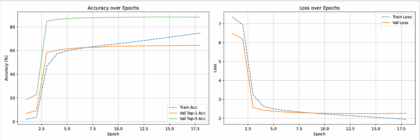
You do not need to just train the classifier of the efficient net model but rather the entire thing. Efficient net is trained on the image net database which contains over a million images covering 1,000 object categories not really characters so it might help to start from the beginning.

Also, It is mathematically true to have a higher top 5 accuracy than top 1 but the model seems to be doing terrible (depending if your data is similar to mine)

My dataset is similar but might not be the exact same (processed version of ETL9G data). It has 3036 characters, 607,000 images, ~200 images per class and is based on ocr.

To hyperoptimize you might need complex things like arc face, TTA.

It is nothing wrong with the actual models *my experiments showed high results using a similar sized dataset ( ETL9G_images_processed_96x96 | Kaggle )

So I ran my own experiment with this code (full google drive link: Google Colab ).

\!pip install -q timm 'torchvision>=0.15.0' japanize-matplotlib
\!pip install -q kaggle

import os
from google.colab import files

# upload your kaggle.json privately for dataset download
print("Please upload your kaggle.json file:")
uploaded = files.upload()

if 'kaggle.json' in uploaded:
    !mkdir -p ~/.kaggle
    !cp kaggle.json ~/.kaggle/
    !chmod 600 ~/.kaggle/kaggle.json
    print("Kaggle API key configured successfully.")

    # download a publicly available pre-processed ETL9G dataset
    !kaggle datasets download -d votrancong/etl9g-images-processed-96x96

    print("Unzipping ETL9G Dataset...")
    !unzip -q etl9g-images-processed-96x96.zip -d ./etl9g_data
    print("Dataset ready!")
else:
    print("Please upload the kaggle.json file to proceed.")

import torch
import numpy as np
import matplotlib.pyplot as plt

# renders Kanji cleanly in plots
import japanize_matplotlib
from torch.utils.data import DataLoader, random_split
from torchvision.datasets import ImageFolder
from torchvision.transforms import v2

train_transforms = v2.Compose([
    v2.ToImage(),
    v2.ToDtype(torch.float32, scale=True),
    v2.RandomResizedCrop(size=(64, 64), scale=(0.8, 1.0)),
    v2.RandomRotation(degrees=10),
    v2.RandomAffine(degrees=0, shear=10, translate=(0.1, 0.1)),
    v2.ElasticTransform(alpha=25.0),
    v2.GaussianBlur(kernel_size=3, sigma=(0.1, 1.2)),
    v2.RandomErasing(p=0.3),
    v2.Grayscale(num_output_channels=1),
    v2.Normalize(mean=[0.5], std=[0.5])
])

val_transforms = v2.Compose([
    v2.ToImage(),
    v2.ToDtype(torch.float32, scale=True),
    v2.Resize((64, 64)),
    v2.Grayscale(num_output_channels=1),
    v2.Normalize(mean=[0.5], std=[0.5])
])

data_dir = './etl9g_data/images_progressed/'
full_dataset = ImageFolder(root=data_dir)

# split into 80 train 20 val
train_size = int(0.8 * len(full_dataset))
val_size = len(full_dataset) - train_size
train_dataset, val_dataset = random_split(full_dataset, [train_size, val_size])

# apply respective transforms
train_dataset.dataset.transform = train_transforms
val_dataset.dataset.transform = val_transforms

# this is small for an a100 but too late
batch_size = 1024
train_loader = DataLoader(train_dataset, batch_size=batch_size, shuffle=True, num_workers=4, pin_memory=True, persistent_workers=True)
val_loader = DataLoader(val_dataset, batch_size=batch_size, shuffle=False, num_workers=4, pin_memory=True, persistent_workers=True)

print(f"Total Classes: {len(full_dataset.classes)}")
print(f"Training Samples: {train_size} | Validation Samples: {val_size}")

# chart 1 of Class Distribution

class_counts = np.bincount([target for _, target in full_dataset.samples])

plt.figure(figsize=(12, 4))
plt.bar(range(len(class_counts)), class_counts, width=1.0, color='royalblue')
plt.title("ETL9G Class Distribution")
plt.xlabel("Class Index")
plt.ylabel("Number of Samples")
plt.show()

# chart 2 of visualizing some augmented samples
def show_batch(dataloader, classes):
    images, labels = next(iter(dataloader))
    plt.figure(figsize=(10, 10))
    for i in range(9):
        ax = plt.subplot(3, 3, i + 1)
        # denormalize image
        img = images[i].numpy().squeeze() * 0.5 + 0.5
        plt.imshow(img, cmap="gray")
        plt.title(classes[labels[i].item()], fontsize=16)
        plt.axis("off")
    plt.tight_layout()
    plt.show()

print("\nAugmented Training Samples:")
show_batch(train_loader, full_dataset.classes)

import timm
import torch.nn as nn

device = torch.device("cuda" if torch.cuda.is_available() else "cpu")
print(f"Using device: {device}")

# create "EfficientNet-Lite0" using timm
# in_chans=1 automatically adapts the first conv layer for grayscale
num_classes = len(full_dataset.classes)
model = timm.create_model(
    'efficientnet_lite0',
    pretrained=False,
    in_chans=1,
    num_classes=num_classes
)

model = model.to(device)

import torch
import torch.nn as nn
import torch.optim as optim
import matplotlib.pyplot as plt
from tqdm.auto import tqdm

# enable TF32 for massive speedups in FP32 operations without code changes
torch.backends.cuda.matmul.allow_tf32 = True
torch.backends.cudnn.allow_tf32 = True


# helper func for top-1 / top-5 accuracy
def calculate_topk_accuracy(output, target, topk=(1, 5)):
    with torch.no_grad():
        maxk = max(topk)
        _, pred = output.topk(maxk, 1, True, True)
        pred = pred.t()
        correct = pred.eq(target.view(1, -1).expand_as(pred))

        res = []
        for k in topk:
            correct_k = correct[:k].reshape(-1).float().sum(0, keepdim=True)
            res.append(correct_k.item())
        return res


epochs = 5
learning_rate = 1e-3


# more optimizations
model = torch.compile(model)

optimizer = optim.AdamW(model.parameters(), lr=learning_rate, weight_decay=1e-4)
scheduler = optim.lr_scheduler.CosineAnnealingLR(optimizer, T_max=epochs)
criterion = nn.CrossEntropyLoss()

# no GradScaler cuz bfloat16 handles ranges natively
best_val_acc = 0.0

history = {
    'train_loss': [], 'val_loss': [],
    'train_top1': [], 'val_top1': [],
    'train_top5': [], 'val_top5': []
}

for epoch in range(epochs):

    model.train()
    train_loss, train_total = 0.0, 0
    train_correct_top1, train_correct_top5 = 0.0, 0.0

    pbar = tqdm(train_loader, desc=f"Epoch {epoch+1}/{epochs} [Train]")
    for images, labels in pbar:

        images = images.to(device, non_blocking=True)
        labels = labels.to(device, non_blocking=True)

        optimizer.zero_grad(set_to_none=True)

        # im using a A100 which natively supports bf16.
        # It avoids the underflow/overflow issues of fp16.
        with torch.autocast(device_type='cuda', dtype=torch.bfloat16):
            outputs = model(images)
            loss = criterion(outputs, labels)


        loss.backward()
        optimizer.step()

        train_loss += loss.item() * images.size(0)
        train_total += labels.size(0)

        acc1, acc5 = calculate_topk_accuracy(outputs, labels, topk=(1, 5))
        train_correct_top1 += acc1
        train_correct_top5 += acc5

        pbar.set_postfix({
            'loss': f"{loss.item():.4f}",
            'top1': f"{train_correct_top1/train_total:.4f}",
            'top5': f"{train_correct_top5/train_total:.4f}"
        })

    scheduler.step()

    # calc average training metrics
    epoch_train_loss = train_loss / train_total
    epoch_train_top1 = train_correct_top1 / train_total
    epoch_train_top5 = train_correct_top5 / train_total

    history['train_loss'].append(epoch_train_loss)
    history['train_top1'].append(epoch_train_top1)
    history['train_top5'].append(epoch_train_top5)

    model.eval()
    val_loss, val_total = 0.0, 0
    val_correct_top1, val_correct_top5 = 0.0, 0.0

    with torch.no_grad():
        for images, labels in tqdm(val_loader, desc=f"Epoch {epoch+1}/{epochs}   [Val]"):
            images = images.to(device, non_blocking=True)
            labels = labels.to(device, non_blocking=True)

            with torch.autocast(device_type='cuda', dtype=torch.bfloat16):
                outputs = model(images)
                loss = criterion(outputs, labels)

            val_loss += loss.item() * images.size(0)
            val_total += labels.size(0)

            acc1, acc5 = calculate_topk_accuracy(outputs, labels, topk=(1, 5))
            val_correct_top1 += acc1
            val_correct_top5 += acc5

    epoch_val_loss = val_loss / val_total
    epoch_val_top1 = val_correct_top1 / val_total
    epoch_val_top5 = val_correct_top5 / val_total

    history['val_loss'].append(epoch_val_loss)
    history['val_top1'].append(epoch_val_top1)
    history['val_top5'].append(epoch_val_top5)

    print(f"Train Loss: {epoch_train_loss:.4f} | Val Loss: {epoch_val_loss:.4f}")
    print(f"Train Top-1: {epoch_train_top1:.4f} | Val Top-1: {epoch_val_top1:.4f}")
    print(f"Train Top-5: {epoch_train_top5:.4f} | Val Top-5: {epoch_val_top5:.4f}")

    if epoch_val_top1 > best_val_acc:
        best_val_acc = epoch_val_top1
        torch.save(model.state_dict(), "best_kanji_efficientnet_lite0.pth")
        print("--> Saved Best Model!")

# Plotting stuff
plt.figure(figsize=(15, 5))

# Loss
plt.subplot(1, 3, 1)
plt.plot(history['train_loss'], label='Train Loss')
plt.plot(history['val_loss'], label='Val Loss')
plt.title('Loss over Epochs')
plt.xlabel('Epochs')
plt.ylabel('Loss')
plt.legend()
plt.grid(True)

# Top-1 Accuracy over epochs
plt.subplot(1, 3, 2)
plt.plot(history['train_top1'], label='Train Top-1 Acc')
plt.plot(history['val_top1'], label='Val Top-1 Acc')
plt.title('Top-1 Accuracy over Epochs')
plt.xlabel('Epochs')
plt.ylabel('Accuracy')
plt.legend()
plt.grid(True)

# Top-5 Accuracy over epochs
plt.subplot(1, 3, 3)
plt.plot(history['train_top5'], label='Train Top-5 Acc')
plt.plot(history['val_top5'], label='Val Top-5 Acc')
plt.title('Top-5 Accuracy over Epochs')
plt.xlabel('Epochs')
plt.ylabel('Accuracy')
plt.legend()
plt.grid(True)

plt.tight_layout()
plt.show()

Epoch 1/5 [Train]: 100%

452/452 [04:23<00:00, 14.97s/it, loss=2.2282, top1=0.0974, top5=0.2323]

Epoch 1/5   [Val]: 100%

113/113 [00:55<00:00,  3.51it/s]

Train Loss: 5.3181 | Val Loss: 2.4894
Train Top-1: 0.0974 | Val Top-1: 0.3684
Train Top-5: 0.2323 | Val Top-5: 0.7049

Epoch 2/5 [Train]: 100%

452/452 [02:10<00:00,  3.18it/s, loss=0.6743, top1=0.6817, top5=0.9166]

Epoch 2/5   [Val]: 100%

113/113 [00:34<00:00,  3.86it/s]

Train Loss: 1.1602 | Val Loss: 0.7087
Train Top-1: 0.6817 | Val Top-1: 0.7945
Train Top-5: 0.9166 | Val Top-5: 0.9646

Epoch 3/5 [Train]: 100%

452/452 [02:10<00:00,  5.10it/s, loss=0.4238, top1=0.8798, top5=0.9848]

Epoch 3/5   [Val]: 100%

113/113 [00:35<00:00,  3.53it/s]

Train Loss: 0.4149 | Val Loss: 0.4418
Train Top-1: 0.8798 | Val Top-1: 0.8710
Train Top-5: 0.9848 | Val Top-5: 0.9818


Epoch 4/5 [Train]: 100%

452/452 [02:12<00:00,  3.02it/s, loss=0.2243, top1=0.9399, top5=0.9946]

Epoch 4/5   [Val]: 100%

113/113 [00:35<00:00,  3.16it/s]

Train Loss: 0.2130 | Val Loss: 0.2990
Train Top-1: 0.9399 | Val Top-1: 0.9138
Train Top-5: 0.9946 | Val Top-5: 0.9895


Epoch 5/5 [Train]: 100%

452/452 [02:10<00:00,  4.00it/s, loss=0.1319, top1=0.9692, top5=0.9978]

Epoch 5/5   [Val]: 100%

113/113 [00:35<00:00,  3.32it/s]

Train Loss: 0.1245 | Val Loss: 0.2424
Train Top-1: 0.9692 | Val Top-1: 0.9311
Train Top-5: 0.9978 | Val Top-5: 0.9912

Here is the efficent net b0 model which uses pretrained efficientnet_b0 converges even faster by epoch 2 (Heres the link for that one ( Google Colab )).

All i changed was this

model = timm.create_model('efficientnet_b0', pretrained=True, in_chans=1, num_classes=num_classes)

Epoch 1/2 [Train]: 100%

452/452 [02:53<00:00,  3.44it/s, loss=0.2283, top1=0.7560, top5=0.8551]

Epoch 1/2   [Val]: 100%

113/113 [00:45<00:00,  3.13it/s]

Train Loss: 1.3734 | Val Loss: 0.1795
Train Top-1: 0.7560 | Val Top-1: 0.9502
Train Top-5: 0.8551 | Val Top-5: 0.9955


Epoch 2/2 [Train]: 100%

452/452 [02:58<00:00,  2.72it/s, loss=0.0792, top1=0.9827, top5=0.9991]

Epoch 2/2   [Val]: 100%

113/113 [00:44<00:00,  2.58it/s]

Train Loss: 0.0672 | Val Loss: 0.0969
Train Top-1: 0.9827 | Val Top-1: 0.9732
Train Top-5: 0.9991 | Val Top-5: 0.9978

[Marco]

Wow, thanks for this detailed explanation!
I already suspected that maybe my model setup was not correct for this use case.