I am developing a model where, for some technical reasons, my minimization objective is actually the squared norm of the gradient of some loss function:
In the following toy example, I am implementing this for a very simple case (least-squares linear regression from the 2-dimensional space to the 1-dimensional space):
import torch
from torch import Tensor
from torch.autograd import Variable
from torch import nn

# some toy data
x = Variable(Tensor([4., 2.]), requires_grad=False)
y = Variable(Tensor([1.]), requires_grad=False)

# linear model and squared difference loss
model = nn.Linear(2, 1)
loss = torch.sum((y - model(x))**2)

# first backward pass
model.zero_grad()
# set create_graph=True to allow the computation of higher order derivatives afterwards
loss.backward(create_graph=True)

# compute the squared norm of the loss gradient
gn2 = Variable(Tensor([0.]))
for param in model.parameters():
  gn2 = gn2 + param.grad.norm()**2

# we do not want to accumulate the previous gradients with the new ones,
# so we have to call zero_grad() again
model.zero_grad()
gn2.backward()
However, PyTorch complains about backpropagating through variables that were modified by inplace operations:
RuntimeError: one of the variables needed for gradient computation has been modified by an inplace operation
After some debug, I found out that the second call to model.zero_grad() is responsible for that error, because it sets gradients to zero using inplace operations. An obvious (but maybe inelegant?) workaround is manually “zeroing” the gradients in the for loop and removing the second call to model.zero_grad(), that is, doing:
...
# compute the squared norm of the loss gradient
gn2 = Variable(Tensor([0.]))
for param in model.parameters():
  gn2 = gn2 + param.grad.norm()**2
  param.grad = torch.zeros_like(param)

gn2.backward()
Everything would be cleaner if the function zero_grad() had an inplace argument, that we could set to False in situations like this…
What do you think? Which is the correct way to deal with this situation?
This is my code following your suggestion, in case anyone else comes across this problem and finds it useful:
import torch
from torch import Tensor
from torch.autograd import Variable
from torch.autograd import grad
from torch import nn

# some toy data
x = Variable(Tensor([4., 2.]), requires_grad=False)
y = Variable(Tensor([1.]), requires_grad=False)

# linear model and squared difference loss
model = nn.Linear(2, 1)
loss = torch.sum((y - model(x))**2)

# instead of using loss.backward(), use torch.autograd.grad() to compute gradients
loss_grads = grad(loss, model.parameters(), create_graph=True)

# compute the squared norm of the loss gradient
gn2 = sum([grd.norm()**2 for grd in loss_grads])

model.zero_grad()
gn2.backward()
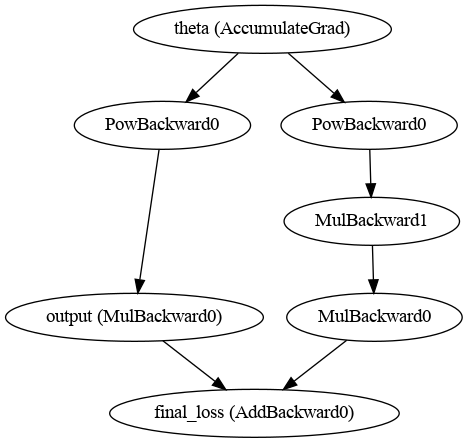
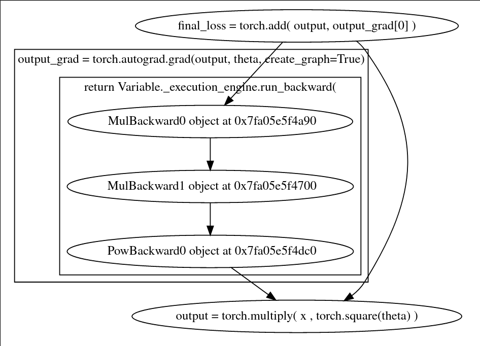
I am hopelessly trying to figure out how the computational graph would look like with second derivatives involved. I understand how auto diff works in 1st order derivative case and can work my way with drawing the computational graph. But for higher-order derivatives, I simply cannot do so.
I can only find the code on how this can be done in the internet but not an exact figurative answer. This is the closest answer I could find, but still, didn’t quite get it.
Ha! I could spend hours with this (in fact I did record an entire course on autograd, but I don’t want to spam the forum with advertisement), but so the short story is two things on this:
As mentioned above, I strongly advocate to never use create_graph with t.backward but only ever use it with torch.autograd.grad. t.backward is a convenience function that computes gradients and accumulates them in .grad. You almost certainly don’t want that to happen with the bits you take second derivatives of, and it creates all sorts of issues (e.g. with circular references).
Remember that inside the backward of an autograd function, you are using normal PyTorch operations. In this sense an oversimplified explanation of higher order derivatives is that all that create_graph does is to enable requires_grad=True in the backward. This should help you to draw the graph (adding to the computational graph you had in the forward while you are computing the gradient from the initial forward).
If I am not asking too much, could you post a rough hand-drawn picture of how the computational graph for this code below would look like. And please do share the link of your auto-grad course. : robinnarsingha123 at gmail dot com
I’m sorry to open such an old question, but I did have some difficulties. I need to add gradient L1 regularization to my loss, and I find that only the following two times backward implementation can make its update result different from the result without gradient regularization. If, as you suggested, torch.autograd.grad is used to replace the first backward, the updated result is the same as the result without gradient regularization, I don’t know why this happens. And whether the two backward implementation would actually work as I hoped.
the code of toy:
import torch
x = torch.randn(3,4)
fc1 = torch.nn.Linear(4,3)
fc2 = torch.nn.Linear(4,3)
fc3 = torch.nn.Linear(4,3)
fc2.weight.data.copy_(fc1.weight.data)
fc2.bias.data.copy_(fc1.bias.data)
fc3.weight.data.copy_(fc1.weight.data)
fc3.bias.data.copy_(fc1.bias.data)
opt1 = torch.optim.SGD(fc1.parameters(), lr=0.01)
opt2 = torch.optim.SGD(fc2.parameters(), lr=0.01)
opt3 = torch.optim.SGD(fc3.parameters(), lr=0.01)

# without gradient regularization
y1 = fc1(x)
loss1 = (1-y1).sum()
loss1.backward()
opt1.step()

# with gradient regularization, first implementation
y2 = fc2(x)
l2 = (1-y2).sum()
l2.backward(create_graph=True)
np2 = sum([p.grad.norm(p=1) for p in fc2.parameters()])
loss2 = l2 + np2
loss2.backward()
opt2.step()

# with gradient regularization, second implementation
y3 = fc3(x)
l3 = (1-y3).sum()
np3 = sum([g.norm(p=1) for g in  torch.autograd.grad(l3, fc3.parameters(), create_graph=True) ])
loss3 = l3 + np3
loss3.backward()
opt3.step()

# print weight after update
print(fc1.weight)
print(fc2.weight)  # different to fc1.weight
print(fc3.weight)  # same to fc1.weight
I seem to know where I went wrong. The second derivative of the linear function is 0, which makes torch.autograd.grad same to without gradients norm, but not if I make it be nonlinear function.
Looks like the torch.autograd.grad implementation is the right one? If anyone can help confirm would be greatly appreciated!