I am not able to build a custom learning rate scheduler using SequentialLR. To elaborate, I am trying to combine CosineAnnealingLR followed by ConstantLR (as per the code below).
I have set the initial learning rate of 0.1
- I was expecting to have a cosine decay starting from the learning rate of 0.1 and decay to 1e-4 for first 72 epochs
- Thereafter, for last 18 epochs, I would like to have a fixed learning rate of 1e-4
import torch
import math
from torch.optim.lr_scheduler import SequentialLR, CosineAnnealingLR, ConstantLR
from matplotlib import pyplot as plt

class TinyModel(torch.nn.Module):
    def __init__(self):
        super(TinyModel, self).__init__()
        self.linear2 = torch.nn.Linear(10, 10)
        self.softmax = torch.nn.Softmax()

    def forward(self, x):
        x = self.linear1(x)
        x = self.softmax(x)
        return x

# Set the parameters for learning
num_epochs = 90

model = TinyModel()

optimizer = torch.optim.SGD(
    params=model.parameters(),
    lr=0.1,
    momentum=0.9,
    weight_decay=5e-5,
)

num_steps_optimizer1 = math.ceil(num_epochs * 0.8)
num_steps_optimizer2 = num_epochs - num_steps_optimizer1

scheduler1 = CosineAnnealingLR(optimizer, T_max=num_steps_optimizer1, eta_min=1e-4)
scheduler2 = ConstantLR(optimizer, factor=1e-3, total_iters=num_steps_optimizer2)
scheduler = SequentialLR(optimizer, schedulers=[scheduler1, scheduler2], milestones=[num_steps_optimizer1+1])

lr_schedule = []
for epoch in range(num_epochs):
    # train_epoch(...)
    scheduler.step()
    lr_schedule.extend(scheduler.get_last_lr())

# plotting the simulated LR schedule
plt.figure(figsize=(5, 3))
plt.plot(range(len(lr_schedule)), lr_schedule)
plt.xlabel('Epochs')
plt.ylabel('Learning rate')
plt.tight_layout()
plt.show()
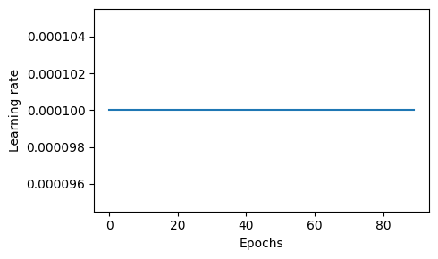
The issue with my implementation is that, the initial learning rate of the CosineAnnealingLR is being determined by the factor that I set for ConstantLR.
More precisely, I observe the following:
with the setting,
scheduler1 = CosineAnnealingLR(optimizer, T_max=num_steps_optimizer1, eta_min=1e-4)
scheduler2 = ConstantLR(optimizer, factor=1e-3, total_iters=num_steps_optimizer2)
I notice the following plot:
and, with the following setting (changed the eta_min in scheduler1),
scheduler1 = CosineAnnealingLR(optimizer, T_max=num_steps_optimizer1, eta_min=1e-5)
scheduler2 = ConstantLR(optimizer, factor=1e-3, total_iters=num_steps_optimizer2)
I notice the following plot:
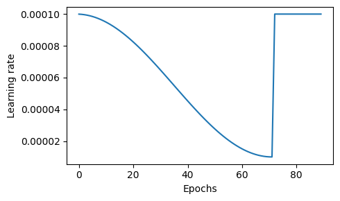
So therefore, I conclude that the factor parameter in scheduler2 is influencing the initial learning rate for scheduler1.
I would appreciate any insights and guidance on how to overcome this issue.