The code is below:
import torch
import matplotlib.pyplot as plt
from torch.autograd import Variable

# torch.manual_seed(1)    # reproducible

N_SAMPLES = 20
N_HIDDEN = 300

# training data
x = torch.unsqueeze(torch.linspace(-1, 1, N_SAMPLES), 1)
y = x + 0.3*torch.normal(torch.zeros(N_SAMPLES, 1), torch.ones(N_SAMPLES, 1))

x = Variable(x)
y = Variable(y)

# test data
test_x = torch.unsqueeze(torch.linspace(-1, 1, N_SAMPLES), 1)
test_y = test_x + 0.3*torch.normal(torch.zeros(N_SAMPLES, 1), torch.ones(N_SAMPLES, 1))

test_x = Variable(test_x)
test_y = Variable(test_y)

# show data
plt.scatter(x.data.numpy(), y.data.numpy(), c='magenta', s=50, alpha=0.5, label='train')
plt.scatter(test_x.data.numpy(), test_y.data.numpy(), c='cyan', s=50, alpha=0.5, label='test')
plt.legend(loc='upper left')
plt.ylim((-2.5, 2.5))
plt.show()

net_overfitting = torch.nn.Sequential(
    torch.nn.Linear(1, N_HIDDEN),
    torch.nn.ReLU(),
    torch.nn.Linear(N_HIDDEN, N_HIDDEN),
    torch.nn.ReLU(),
    torch.nn.Linear(N_HIDDEN, 1),
)

net_dropped = torch.nn.Sequential(
    torch.nn.Linear(1, N_HIDDEN),
    torch.nn.Dropout(0.5),  # drop 50% of the neuron
    torch.nn.ReLU(),
    torch.nn.Linear(N_HIDDEN, N_HIDDEN),
    torch.nn.Dropout(0.5),  # drop 50% of the neuron
    torch.nn.ReLU(),
    torch.nn.Linear(N_HIDDEN, 1),
)

print(net_overfitting)  # net architecture
print(net_dropped)

optimizer_ofit = torch.optim.Adam(net_overfitting.parameters(), lr=0.01)
optimizer_drop = torch.optim.Adam(net_dropped.parameters(), lr=0.01)
loss_func = torch.nn.MSELoss()

plt.ion()   # something about plotting

for t in range(500):
    pred_ofit = net_overfitting(x)
    pred_drop = net_dropped(x)
    loss_ofit = loss_func(pred_ofit, y)
    loss_drop = loss_func(pred_drop, y)

    optimizer_ofit.zero_grad()
    optimizer_drop.zero_grad()
    loss_ofit.backward()
    loss_drop.backward()
    optimizer_ofit.step()
    optimizer_drop.step()

    if t % 10 == 0:
        # change to eval mode in order to fix drop out effect
        net_overfitting.eval()
        net_dropped.eval()  # parameters for dropout differ from train mode

        # plotting
        plt.cla()
        test_pred_ofit = net_overfitting(test_x)
        test_pred_drop = net_dropped(test_x)
        plt.scatter(x.data.numpy(), y.data.numpy(), c='magenta', s=50, alpha=0.3, label='train')
        plt.scatter(test_x.data.numpy(), test_y.data.numpy(), c='cyan', s=50, alpha=0.3, label='test')
        plt.plot(test_x.data.numpy(), test_pred_ofit.data.numpy(), 'r-', lw=3, label='overfitting')
        plt.plot(test_x.data.numpy(), test_pred_drop.data.numpy(), 'b--', lw=3, label='dropout(50%)')
        plt.text(0, -1.2, 'overfitting loss=%.4f' % loss_func(test_pred_ofit, test_y).data.numpy(), fontdict={'size': 20, 'color':  'red'})
        plt.text(0, -1.5, 'dropout loss=%.4f' % loss_func(test_pred_drop, test_y).data.numpy(), fontdict={'size': 20, 'color': 'blue'})
        plt.legend(loc='upper left'); plt.ylim((-2.5, 2.5));plt.pause(0.1)

        # change back to train mode
        net_overfitting.train()
        net_dropped.train()

plt.ioff()
Run this program and get the following result:
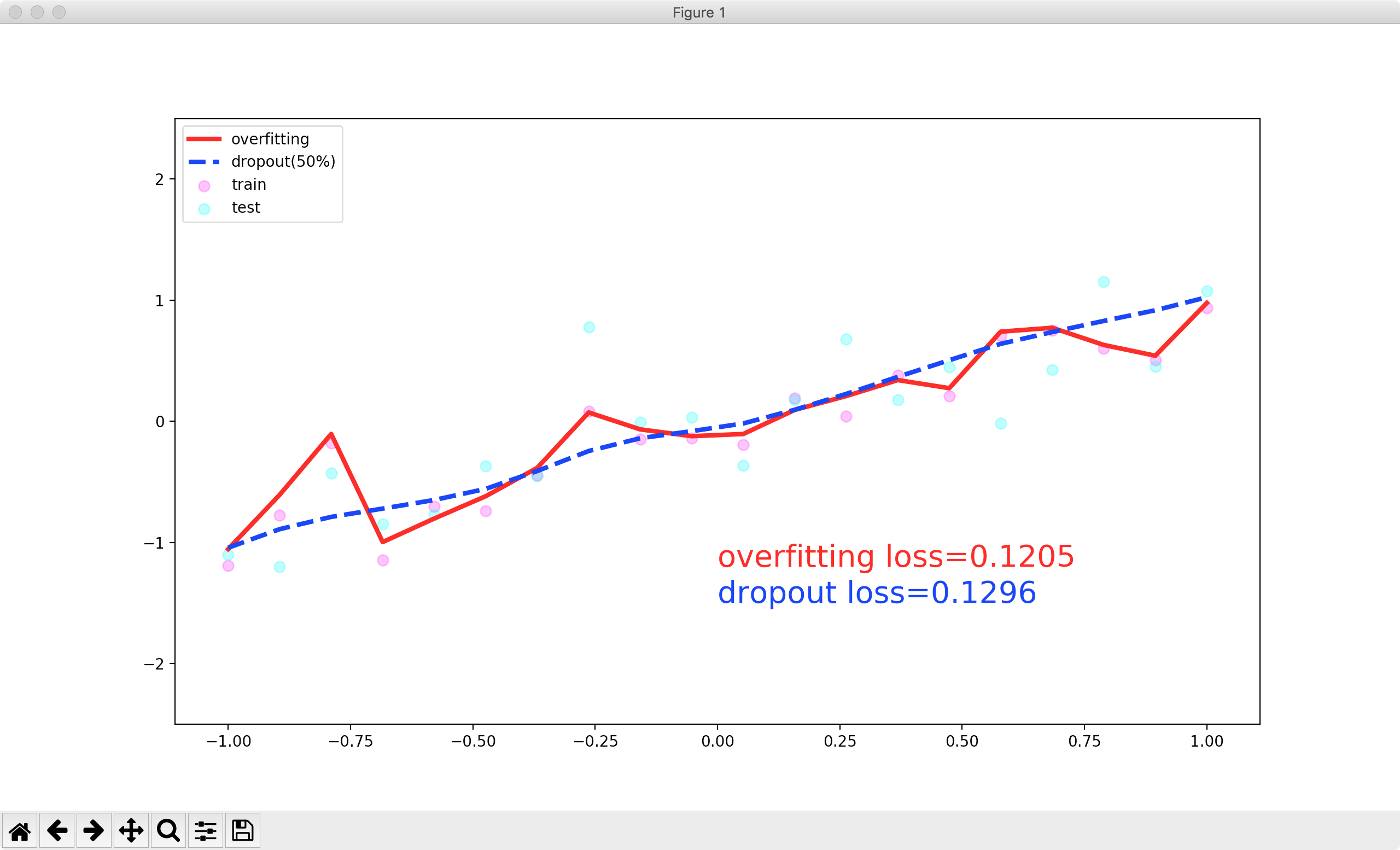
Here is my question:
1.what is valuation model?Why should I use these two lines of code to enter the evaluation mode?
net_overfitting.eval()
net_dropped.eval()
- Is the curve above for the training set or the test set?
Through the image, it can be seen that the curve is probably fitted by the training set.But the code is written like this:
plt.plot(test_x.data.numpy(), test_pred_ofit.data.numpy(), 'r-', lw=3, label='overfitting')
plt.plot(test_x.data.numpy(), test_pred_drop.data.numpy(), 'b--', lw=3, label='dropout(50%)')
So I am very confused, who can tell me what is going on, why is this, thank you very much!
I hope to get a detailed answer, thank you very much!