Hi all, I’m very new here (and to deep learning!) so apologies in advance for the inevitably poor formatting, description and long-winded post ahead.
I am trying to replicate some code form two repositories, one of which is written in pytorch, the other in tensorflow:
I have modified the code slightly so that (1) is now solving the same problem as (2), explicitly the code is just implementing the method outlined here: (ahttps://arxiv.org/abs/1708.07469) and I am trying to use it for solving a finance problem (pricing a European call option), though this isn’t particularly important. It is also worth stating here that the tensorflow code was written using version 1.14, hence I have had to downgrade my tensorflow package to use it as is.
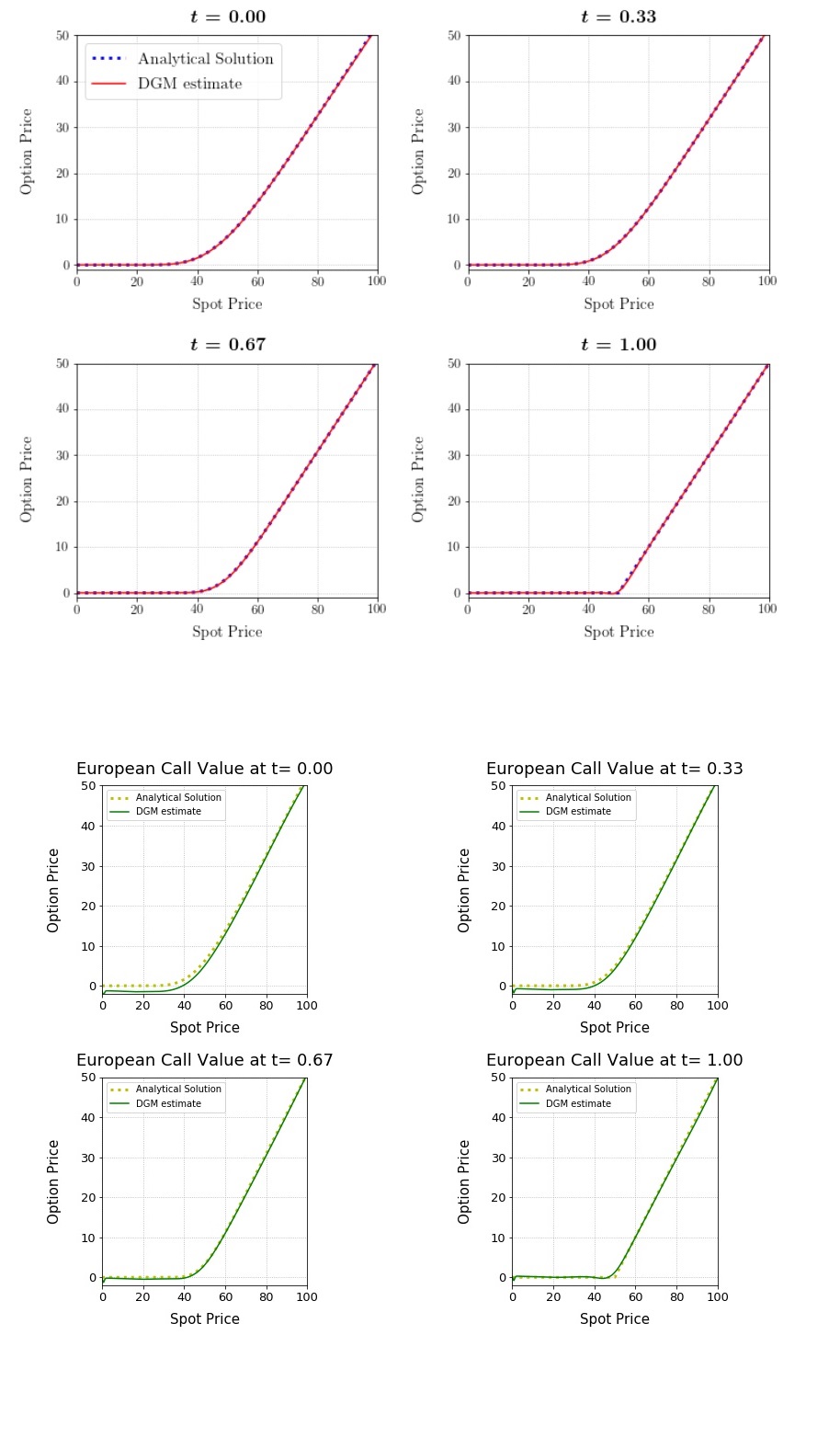
The tensorflow network gives excellent results (L2-Norm of approximately 0.001 after 500 epochs) whilst the ‘identical’ network in pytorch converges much less rapidly and struggles to achieve a loss value below 1-2. I am hesitant to think that this is an issue relating to ahttps://discuss.pytorch.org/t/suboptimal-convergence-when-compared-with-tensorflow-model/5099 (apologies for the formatting, 2 links only for new users) or (ahttps://discuss.pytorch.org/t/the-same-model-produces-worse-results-on-pytorch-than-on-tensorflow/5380), mainly because I am massively inexperienced (hence I’ve probably overlooked something) and because a similar post (ahttps://discuss.pytorch.org/t/pytorch-adam-vs-tensorflow-adam/74471)) indicated that it was a coding problem rather than a framework problem.
I will include all of the raw code below (apologies in advance) and I have included some figures showing the discrepancy in the final results.
Hopefully someone will be able to untangle me from this mess and I thank you all in advance for your patience with this post!
Tensorflow Code:
#%% import needed packages
import tensorflow as tf


#%% LSTM-like layer used in DGM (see Figure 5.3 and set of equations on p. 45) - modification of Keras layer class

class LSTMLayer(tf.keras.layers.Layer):

    # constructor/initializer function (automatically called when new instance of class is created)
    def __init__(self, output_dim, input_dim, trans1 = "tanh", trans2 = "tanh"):
        '''
        Args:
            input_dim (int):       dimensionality of input data
            output_dim (int):      number of outputs for LSTM layers
            trans1, trans2 (str):  activation functions used inside the layer;
                                   one of: "tanh" (default), "relu" or "sigmoid"

        Returns: customized Keras layer object used as intermediate layers in DGM
        '''

        # create an instance of a Layer object (call initialize function of superclass of LSTMLayer)
        super(LSTMLayer, self).__init__()

        # add properties for layer including activation functions used inside the layer
        self.output_dim = output_dim
        self.input_dim = input_dim

        if trans1 == "tanh":
            self.trans1 = tf.nn.tanh
        elif trans1 == "relu":
            self.trans1 = tf.nn.relu
        elif trans1 == "sigmoid":
            self.trans1 = tf.nn.sigmoid

        if trans2 == "tanh":
            self.trans2 = tf.nn.tanh
        elif trans2 == "relu":
            self.trans2 = tf.nn.relu
        elif trans2 == "sigmoid":
            self.trans2 = tf.nn.relu

        ### define LSTM layer parameters (use Xavier initialization)
        # u vectors (weighting vectors for inputs original inputs x)
        self.Uz = self.add_variable("Uz", shape=[self.input_dim, self.output_dim],
                                    initializer = tf.contrib.layers.xavier_initializer())
        self.Ug = self.add_variable("Ug", shape=[self.input_dim ,self.output_dim],
                                    initializer = tf.contrib.layers.xavier_initializer())
        self.Ur = self.add_variable("Ur", shape=[self.input_dim, self.output_dim],
                                    initializer = tf.contrib.layers.xavier_initializer())
        self.Uh = self.add_variable("Uh", shape=[self.input_dim, self.output_dim],
                                    initializer = tf.contrib.layers.xavier_initializer())

        # w vectors (weighting vectors for output of previous layer)
        self.Wz = self.add_variable("Wz", shape=[self.output_dim, self.output_dim],
                                    initializer = tf.contrib.layers.xavier_initializer())
        self.Wg = self.add_variable("Wg", shape=[self.output_dim, self.output_dim],
                                    initializer = tf.contrib.layers.xavier_initializer())
        self.Wr = self.add_variable("Wr", shape=[self.output_dim, self.output_dim],
                                    initializer = tf.contrib.layers.xavier_initializer())
        self.Wh = self.add_variable("Wh", shape=[self.output_dim, self.output_dim],
                                    initializer = tf.contrib.layers.xavier_initializer())

        # bias vectors
        self.bz = self.add_variable("bz", shape=[1, self.output_dim])
        self.bg = self.add_variable("bg", shape=[1, self.output_dim])
        self.br = self.add_variable("br", shape=[1, self.output_dim])
        self.bh = self.add_variable("bh", shape=[1, self.output_dim])


    # main function to be called
    def call(self, S, X):
        '''Compute output of a LSTMLayer for a given inputs S,X .
        Args:
            S: output of previous layer
            X: data input

        Returns: customized Keras layer object used as intermediate layers in DGM
        '''

        # compute components of LSTM layer output (note H uses a separate activation function)
        Z = self.trans1(tf.add(tf.add(tf.matmul(X,self.Uz), tf.matmul(S,self.Wz)), self.bz))
        G = self.trans1(tf.add(tf.add(tf.matmul(X,self.Ug), tf.matmul(S, self.Wg)), self.bg))
        R = self.trans1(tf.add(tf.add(tf.matmul(X,self.Ur), tf.matmul(S, self.Wr)), self.br))

        H = self.trans2(tf.add(tf.add(tf.matmul(X,self.Uh), tf.matmul(tf.multiply(S, R), self.Wh)), self.bh))

        # compute LSTM layer output
        S_new = tf.add(tf.multiply(tf.subtract(tf.ones_like(G), G), H), tf.multiply(Z,S))

        return S_new

#%% Fully connected (dense) layer - modification of Keras layer class

class DenseLayer(tf.keras.layers.Layer):

    # constructor/initializer function (automatically called when new instance of class is created)
    def __init__(self, output_dim, input_dim, transformation=None):
        '''
        Args:
            input_dim:       dimensionality of input data
            output_dim:      number of outputs for dense layer
            transformation:  activation function used inside the layer; using
                             None is equivalent to the identity map

        Returns: customized Keras (fully connected) layer object
        '''

        # create an instance of a Layer object (call initialize function of superclass of DenseLayer)
        super(DenseLayer,self).__init__()
        self.output_dim = output_dim
        self.input_dim = input_dim

        ### define dense layer parameters (use Xavier initialization)
        # w vectors (weighting vectors for output of previous layer)
        self.W = self.add_variable("W", shape=[self.input_dim, self.output_dim],
                                   initializer = tf.contrib.layers.xavier_initializer())

        # bias vectors
        self.b = self.add_variable("b", shape=[1, self.output_dim])

        if transformation:
            if transformation == "tanh":
                self.transformation = tf.tanh
            elif transformation == "relu":
                self.transformation = tf.nn.relu
        else:
            self.transformation = transformation


    # main function to be called
    def call(self,X):
        '''Compute output of a dense layer for a given input X
        Args:
            X: input to layer
        '''

        # compute dense layer output
        S = tf.add(tf.matmul(X, self.W), self.b)

        if self.transformation:
            S = self.transformation(S)

        return S

#%% Neural network architecture used in DGM - modification of Keras Model class

class DGMNet(tf.keras.Model):

    # constructor/initializer function (automatically called when new instance of class is created)
    def __init__(self, layer_width, n_layers, input_dim, final_trans=None):
        '''
        Args:
            layer_width:
            n_layers:    number of intermediate LSTM layers
            input_dim:   spaital dimension of input data (EXCLUDES time dimension)
            final_trans: transformation used in final layer

        Returns: customized Keras model object representing DGM neural network
        '''

        # create an instance of a Model object (call initialize function of superclass of DGMNet)
        super(DGMNet,self).__init__()

        # define initial layer as fully connected
        # NOTE: to account for time inputs we use input_dim+1 as the input dimensionality
        self.initial_layer = DenseLayer(layer_width, input_dim+1, transformation = "tanh")

        # define intermediate LSTM layers
        self.n_layers = n_layers
        self.LSTMLayerList = []

        for _ in range(self.n_layers):
            self.LSTMLayerList.append(LSTMLayer(layer_width, input_dim+1))

        # define final layer as fully connected with a single output (function value)
        self.final_layer = DenseLayer(1, layer_width, transformation = final_trans)


    # main function to be called
    def call(self,t,x):
        '''
        Args:
            t: sampled time inputs
            x: sampled space inputs
        Run the DGM model and obtain fitted function value at the inputs (t,x)
        '''

        # define input vector as time-space pairs
        X = tf.concat([t,x],1)

        # call initial layer
        S = self.initial_layer.call(X)

        # call intermediate LSTM layers
        for i in range(self.n_layers):
            S = self.LSTMLayerList[i].call(S,X)

        # call final LSTM layers
        result = self.final_layer.call(S)

        return result


# SCRIPT FOR SOLVING THE BLACK-SCHOLES EQUATION FOR A EUROPEAN CALL OPTION

#%% import needed packages

import tensorflow as tf
import numpy as np
import scipy.stats as spstats
import matplotlib.pyplot as plt

#%% Parameters

# Option parameters
r = 0.05           # Interest rate
sigma = 0.25       # Volatility
K = 50             # Strike
T = 1              # Terminal time
S0 = 0.5           # Initial price

# Solution parameters (domain on which to solve PDE)
t_low = 0 + 1e-10    # time lower bound
S_low = 0.0 + 1e-10  # spot price lower bound
S_high = 2*K         # spot price upper bound

# neural network parameters
num_layers = 3
nodes_per_layer = 50
learning_rate = 0.001

# Training parameters
sampling_stages  = 800   # number of times to resample new time-space domain points
steps_per_sample = 10    # number of SGD steps to take before re-sampling

# Sampling parameters
nSim_interior = 1000
nSim_terminal = 100
S_multiplier  = 1.5   # multiplier for oversampling i.e. draw S from [S_low, S_high * S_multiplier]

# Plot options
n_plot = 1000  # Points on plot grid for each dimension

# Save options
saveOutput = False
saveName   = 'BlackScholes_EuropeanCall'
saveFigure = False
figureName = 'BlackScholes_EuropeanCall.png'

#%% Black-Scholes European call price

def BlackScholesCall(S, K, r, sigma, t):
    ''' Analytical solution for European call option price under Black-Scholes model

    Args:
        S:     spot price
        K:     strike price
        r:     risk-free interest rate
        sigma: volatility
        t:     time
    '''

    d1 = (np.log(S/K) + (r + sigma**2 / 2) * (T-t))/(sigma * np.sqrt(T-t))
    d2 = d1 - (sigma * np.sqrt(T-t))

    callPrice = S * spstats.norm.cdf(d1) - K * np.exp(-r * (T-t)) * spstats.norm.cdf(d2)

    return callPrice

#%% Sampling function - randomly sample time-space pairs

def sampler(nSim_interior, nSim_terminal):
    ''' Sample time-space points from the function's domain; points are sampled
        uniformly on the interior of the domain, at the initial/terminal time points
        and along the spatial boundary at different time points.

    Args:
        nSim_interior: number of space points in the interior of the function's domain to sample
        nSim_terminal: number of space points at terminal time to sample (terminal condition)
    '''

    # Sampler #1: domain interior
    t_interior = np.random.uniform(low=t_low, high=T, size=[nSim_interior, 1])
    S_interior = np.random.uniform(low=S_low, high=S_high*S_multiplier, size=[nSim_interior, 1])

    # Sampler #2: spatial boundary
        # no spatial boundary condition for this problem

    # Sampler #3: initial/terminal condition
    t_terminal = T * np.ones((nSim_terminal, 1))
    S_terminal = np.random.uniform(low=S_low, high=S_high*S_multiplier, size = [nSim_terminal, 1])

    return t_interior, S_interior, t_terminal, S_terminal

#%% Loss function for Fokker-Planck equation

def loss(model, t_interior, S_interior, t_terminal, S_terminal):
    ''' Compute total loss for training.

    Args:
        model:      DGM model object
        t_interior: sampled time points in the interior of the function's domain
        S_interior: sampled space points in the interior of the function's domain
        t_terminal: sampled time points at terminal point (vector of terminal times)
        S_terminal: sampled space points at terminal time
    '''

    # Loss term #1: PDE
    # compute function value and derivatives at current sampled points
    V = model(t_interior, S_interior)
    V_t = tf.gradients(V, t_interior)[0]
    V_s = tf.gradients(V, S_interior)[0]
    V_ss = tf.gradients(V_s, S_interior)[0]
    diff_V = V_t + 0.5 * sigma**2 * S_interior**2 * V_ss + r * S_interior * V_s - r*V


    # compute average L2-norm of differential operator
    L1 = tf.reduce_mean(tf.square(diff_V))

    # Loss term #2: boundary condition
        # no boundary condition for this problem

    # Loss term #3: initial/terminal condition
    target_payoff = tf.nn.relu(S_terminal - K)
    fitted_payoff = model(t_terminal, S_terminal)

    L3 = tf.reduce_mean( tf.square(fitted_payoff - target_payoff) )

    return L1, L3

#%% Set up network

# initialize DGM model (last input: space dimension = 1)
model = DGMNet(nodes_per_layer, num_layers, 1)

# tensor placeholders (_tnsr suffix indicates tensors)
# inputs (time, space domain interior, space domain at initial time)
t_interior_tnsr = tf.placeholder(tf.float32, [None,1])
S_interior_tnsr = tf.placeholder(tf.float32, [None,1])
t_terminal_tnsr = tf.placeholder(tf.float32, [None,1])
S_terminal_tnsr = tf.placeholder(tf.float32, [None,1])

# loss
L1_tnsr, L3_tnsr = loss(model, t_interior_tnsr, S_interior_tnsr, t_terminal_tnsr, S_terminal_tnsr)
loss_tnsr = L1_tnsr + L3_tnsr

# option value function
V = model(t_interior_tnsr, S_interior_tnsr)

# set optimizer
optimizer = tf.train.AdamOptimizer(learning_rate=learning_rate).minimize(loss_tnsr)

# initialize variables
init_op = tf.global_variables_initializer()

# open session
sess = tf.Session()
sess.run(init_op)

#%% Train network
# for each sampling stage
for i in range(sampling_stages):

    # sample uniformly from the required regions
    t_interior, S_interior, t_terminal, S_terminal = sampler(nSim_interior, nSim_terminal)

    # for a given sample, take the required number of SGD steps
    for _ in range(steps_per_sample):
        loss,L1,L3,_ = sess.run([loss_tnsr, L1_tnsr, L3_tnsr, optimizer],
                                feed_dict = {t_interior_tnsr:t_interior, S_interior_tnsr:S_interior, t_terminal_tnsr:t_terminal, S_terminal_tnsr:S_terminal})

    print(f'Total Loss:{loss} \t Interior L2 Norm:{L1} \t Boundary L2 Norm:{L3} \t Epoch :{i}')

# save outout
if saveOutput:
    saver = tf.train.Saver()
    saver.save(sess, './SavedNets/' + saveName)

#%% Plot results

# LaTeX rendering for text in plots
plt.rc('text', usetex=True)
plt.rc('font', family='serif')

# figure options
plt.figure()
plt.figure(figsize = (12,10))

# time values at which to examine density
valueTimes = [t_low, T/3, 2*T/3, T]

# vector of t and S values for plotting
S_plot = np.linspace(S_low, S_high, n_plot)

for i, curr_t in enumerate(valueTimes):

    # specify subplot
    plt.subplot(2,2,i+1)

    # simulate process at current t
    optionValue = BlackScholesCall(S_plot, K, r, sigma, curr_t)

    # compute normalized density at all x values to plot and current t value
    t_plot = curr_t * np.ones_like(S_plot.reshape(-1,1))
    fitted_optionValue = sess.run([V], feed_dict= {t_interior_tnsr:t_plot, S_interior_tnsr:S_plot.reshape(-1,1)})

    # plot histogram of simulated process values and overlay estimated density
    plt.plot(S_plot, optionValue, color = 'b', label='Analytical Solution', linewidth = 3, linestyle=':')
    plt.plot(S_plot, fitted_optionValue[0], color = 'r', label='DGM estimate')

    # subplot options
    plt.ylim(ymin=-1, ymax=K)
    plt.xlim(xmin=0.0, xmax=S_high)
    plt.xlabel(r"Spot Price", fontsize=15, labelpad=10)
    plt.ylabel(r"Option Price", fontsize=15, labelpad=20)
    plt.title(r"\boldmath{$t$}\textbf{ = %.2f}"%(curr_t), fontsize=18, y=1.03)
    plt.xticks(fontsize=13)
    plt.yticks(fontsize=13)
    plt.grid(linestyle=':')

    if i == 0:
        plt.legend(loc='upper left', prop={'size': 16})

# adjust space between subplots
plt.subplots_adjust(wspace=0.3, hspace=0.4)

if saveFigure:
    plt.savefig(figureName)
Pytorch Code:
import numpy as np


class Sampler:
    def __init__(self, bound_list=[], oversampling=[]):
        """ Definition of a sampler over a domain, the boundary list length have to be pair
            Oversampling allow for stepping out of the boundaries """
        self.bound_list = bound_list
        self.oversampling = oversampling

    def get_sample(self, N):
        dim = len(self.bound_list)//2
        samples = np.empty([N, dim], dtype=np.float32)

        # for ease of writing
        bl = self.bound_list
        os = self.oversampling

        for j in range(dim):
            i = j*2
            samples[:,j] = np.random.uniform(low = bl[i], high = bl[i+1]*os[j], size = N)

        return samples


import time
import torch
import torch.nn as nn
import numpy as np

#from derivatives import gradient, hessian
import matplotlib.pyplot as plt
import math

np.random.seed(42)
torch.manual_seed(42)


class Linear(nn.Module):
    """ Copy of linear module from Pytorch, modified to have a Xavier init,
        TODO : figure out what to do with the bias"""
    def __init__(self, in_features, out_features, bias=True):
        super(Linear, self).__init__()
        self.in_features = in_features
        self.out_features = out_features
        self.weight = torch.nn.Parameter(torch.Tensor(out_features, in_features))
        if bias:
            self.bias = torch.nn.Parameter(torch.Tensor(out_features))
        else:
            self.register_parameter('bias', None)
        self.reset_parameters()
    def reset_parameters(self):
        torch.nn.init.xavier_uniform_(self.weight)
        if self.bias is not None:
            torch.nn.init.uniform_(self.bias, -1, 1) #boundary matter?
    def forward(self, input):
        return torch.nn.functional.linear(input, self.weight, self.bias)
    def extra_repr(self):
        return 'in_features={}, out_features={}, bias={}'.format(
            self.in_features, self.out_features, self.bias is not None
        )
class DGM_layer(nn.Module):
    """ See readme for paper source"""
    def __init__(self, in_features, out_feature, residual=False):
        super(DGM_layer, self).__init__()
        self.residual = residual

        self.Z = Linear(out_feature, out_feature)
        self.UZ = Linear(in_features, out_feature, bias=False)
        self.G = Linear(out_feature, out_feature)
        self.UG = Linear(in_features, out_feature, bias=False)
        self.R = Linear(out_feature, out_feature)
        self.UR = Linear(in_features, out_feature, bias=False)
        self.H = Linear(out_feature, out_feature)
        self.UH = Linear(in_features, out_feature, bias=False)

    def forward(self, x, s):
        z = torch.tanh(self.UZ(x) + self.Z(s))
        g = torch.tanh(self.UG(x) + self.G(s))
        r = torch.tanh(self.UR(x) + self.R(s))
        h = torch.tanh(self.UH(x) + self.H(s * r))
        return (1 - g) * h + z * s


class Net(nn.Module):

    def __init__(self, in_size, out_size, neurons, depth):
        super(Net, self).__init__()
        self.dim = in_size
        self.input_layer = Linear(in_size, neurons)
        self.middle_layer = nn.ModuleList([DGM_layer(in_size, neurons) for i in range(depth)])
        self.final_layer = Linear(neurons, out_size)

    def forward(self, X):
        s = torch.tanh(self.input_layer(X))
        for i, layer in enumerate(self.middle_layer):
            s = torch.tanh(layer(X, s))

        return self.final_layer(s)


import math

# PDE parameters
r = torch.tensor(0.05)            # Interest rate
sigma = torch.tensor(0.25)        # Volatility
strike = 50         # Mean
maturity = 1
S = 50
#lambd = (mu-r)/sigma
#gamma = torch.tensor(1)           # Utility decay

# Time limits
T0 = 0.0 + 1e-10    # Initial time
T  = maturity       # Terminal time
time_osf = 1      # Time oversampling factor

# Space limits
S1 = 0.0 + 1e-10           # Low boundary
S2 = 2*strike              # High boundary
underlying_osf = 1.5       # Underlying ovesampling factor

# Merton's analytical known solution
def analytical_solution(t, s):
    K = strike
    d1 = (np.log(s/K) + (r + sigma**2 / 2) * (T-t))/(sigma * np.sqrt(T-t))
    d2 = d1 - (sigma * np.sqrt(T-t))

    return s * spstats.norm.cdf(d1) - K * np.exp(-r * (T-t)) * spstats.norm.cdf(d2)


def true_loss(sample, u_hat):

    loss = 0

    sample_numpy = sample.detach().numpy()
    u_hat_numpy = u_hat.detach().numpy()

    for i in range(len(sample[:,1])):
        u = analytical_solution(sample_numpy[i,0], sample_numpy[i,1])
        u = u.detach().numpy()
        loss += (u - u_hat_numpy[i])**2

    return loss/len(sample[:,1])

    #return -np.exp(-x*gamma*np.exp(r*(T-t)) - (T-t)*0.5*lambd**2)

def euro_payoff(x,k):
    return max(x-k,0)


s1 = Sampler([T0, T, S1, S2], [1, underlying_osf])
s2 = Sampler([T, T, S1, S2], [1,underlying_osf])

model = Net(2, 1, 50, 3)
opt = torch.optim.Adam(model.parameters(), lr=0.001,eps = 1e-07)
#scheduler = torch.optim.lr_scheduler.ExponentialLR(opt,gamma=0.90)

# Number of samples
NS_1 = 1000
NS_2 = 0
NS_3 = 100

# Training parameters
steps_per_sample = 10
sampling_stages = 500


def Loss(model, sample1, sample2, get_true_loss = False):
    # Loss term #1: PDE
    V = model(sample1)
    grad_V = torch.autograd.grad(V.sum(), sample1, create_graph=True, retain_graph=True)[0]
    V_t = grad_V[:,0]
    V_s = grad_V[:,1]
    V_ss = torch.autograd.grad(V_s.sum(), sample1, create_graph=True, retain_graph=True)[0][:,1]

    f = V_t + 0.5 * sigma**2 * sample1[:,1]**2 * V_ss + r * sample1[:,1] * V_s - r*V

    #print(V_t, V_x, V_xx)
    L1 = torch.mean(torch.pow(f, 2))
    #print_graph(L1.grad_fn, 0)
    # Loss term #2: boundary condition
    L2 = 0.0

    # Loss term #3: initial/terminal condition

    u = model(sample2)
    u_true = torch.empty(len(sample2[:,1])).reshape(-1,1)

    for i in range(len(sample2[:,1])):
        u_true[i] = euro_payoff(sample2[i,1], strike)

    L3 = torch.mean(torch.pow(u - u_true, 2))
    #print_graph(L3.grad_fn, 0)

    true_losses = 0

    #if get_true_loss:
     #   true_losses = true_loss(sample1, V)

    return L1, L2, L3, true_losses


def train_model(model, optimizer, scheduler, num_epochs=100):
    losses=[]
    since = time.time()
    model.train()
    # Set model to training mode

    for epoch in range(num_epochs):
        sample1 = torch.tensor(s1.get_sample(NS_1), requires_grad=True)
        sample2 = torch.tensor(s2.get_sample(NS_3))
        #scheduler.step()

        for i in range(steps_per_sample):
            # zero the parameter gradients
            optimizer.zero_grad()


            L1, L2, L3, true_l2 = Loss(model, sample1, sample2)

            loss = L1 + L2 + L3
            # backward + optimize
            #print_graph(loss.grad_fn,0)
            loss.backward()
            optimizer.step()


        losses.append(loss.data)
        epoch += 1
        if epoch % (num_epochs//num_epochs) == 0:
            print(f'epoch {epoch}, loss {loss.data}, L1 : {L1.data}, L3 : {L3.data}')
            print(f'epoch {epoch}, true loss {true_l2}')

    time_elapsed = time.time() - since
    print(f"Training finished in {time_elapsed:.2f} for {num_epochs}.")
    print(f"The final loss value is {loss.data}")

    return losses

training_losses = train_model(model, opt, scheduler, sampling_stages)
Results (Tensorflow is upper 4 plots in red and blue, Pytorch is latter 4 in green and yellow):