The parameters of the model with custom loss function doesn't upgraded thorough its learning over epochs

Thank you for reading my post.
I’m currently developing the peak detection algorithm using CNN to determine the ideal convolution kernel which is representable as the ideal mother wavelet function that will maximize the peak detection accuracy.

To begin with, I created my own IoU loss function and the simple model and tried to run the learning. The execution itself worked without any errors, but somehow it failed.

The parameters of the model with custom loss function doesn’t upgraded thorough its learning over epochs

My own loss function is described as below.

def IoU(inputs: torch.Tensor, labels: torch.Tensor, 
             smooth: float=0.1, threshold: float = 0.5, alpha: float = 1.0):
  '''
  - alpha: a parameter that sharpen the thresholding.
    if alpha = 1 -> thresholded input is the same as raw input.
  '''

  thresholded_inputs = inputs**alpha / (inputs**alpha + (1 - inputs)**alpha)
  inputs = torch.where(thresholded_inputs < threshold, 0, 1)
  batch_size = inputs.shape[0]

  intersect_tensor = (inputs * labels).view(batch_size, -1)
  intersect = intersect_tensor.sum(-1)

  union_tensor = torch.max(inputs, labels).view(batch_size, -1)
  union = union_tensor.sum(-1)

  iou = (intersect + smooth) / (union + smooth)  # We smooth our devision to avoid 0/0
  iou_score = iou.mean()

  return 1- iou_score

and my training model is,

class MLP(nn.Module):
  def __init__(self):
    super().__init__()
    self.net = nn.Sequential(
        nn.Conv1d(1, 1, kernel_size=32, stride=1, padding=16),
        nn.Linear(257, 256),
        nn.LogSoftmax(1)
    )
  def forward(self, x):
    return self.net(x)

model = MLP()
opt = optim.Adadelta(model.parameters())

# initialization of the kernel of Conv1d
def init_kernel(m):
  if type(m) == nn.Conv1d:
    nn.init.kaiming_normal_(m.weight)
    print(m.weight)
    plt.plot(m.weight[0][0].detach().numpy())

model.apply(init_kernel)

def step(x, y, is_train=True):
  opt.zero_grad()

  y_pred = model(x)
  y_pred = y_pred.reshape(-1, 256)

  loss = IoU(y_pred, y)
  loss.requires_grad = True
  loss.retain_grad = True

  if is_train:
    loss.backward()
    opt.step()

  return loss, y_pred

and lastly, the execution code is,

from torch.autograd.grad_mode import F

train_loss_arr, val_loss_arr = [], []
valbose = 10
epochs = 200

for e in range(epochs):
  train_loss, val_loss, acc = 0., 0., 0.,
  for x, y in train_set.as_numpy_iterator():
    x = torch.from_numpy(x)
    y = torch.from_numpy(y)
    model.train()
    loss, y_pred = step(x, y, is_train=True)
    train_loss += loss.item()
  train_loss /= len(train_set)

  for x, y ,in val_set.as_numpy_iterator():
    x = torch.from_numpy(x)
    y = torch.from_numpy(y)
    model.eval()
    with torch.no_grad():
      loss, y_pred = step(x, y, is_train=False)
    val_loss += loss.item()
  val_loss /= len(val_set)

  train_loss_arr.append(train_loss)
  val_loss_arr.append(val_loss)

  # visualize current kernel to check whether the learning is on progress safely.
  if e % valbose == 0: 
    print(f"Epoch[{e}]({(e*100/epochs):0.2f}%):  train_loss: {train_loss:0.4f}, val_loss: {val_loss:0.4f}")
    fig, axs = plt.subplots(1, 4, figsize=(12, 4))
    print(y_pred[0], y_pred[0].shape)
    axs[0].plot(x[0][0])
    axs[0].set_title("spectra")
    axs[1].plot(y_pred[0])
    axs[1].set_title("y pred")
    axs[2].plot(y[0])
    axs[2].set_title("y true")
    axs[3].plot(model.state_dict()["net.0.weight"][0][0].numpy())
    axs[3].set_title("kernel1")
    plt.show()

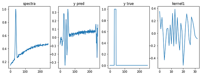
with these programs, I tried to evaluate this simple model, however, model parameters didn’t change at all over epochs.

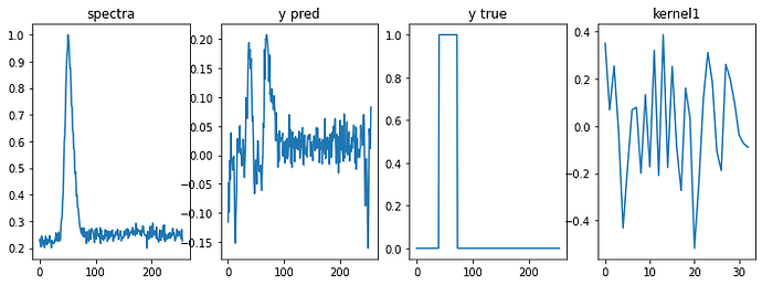
Visualization of the results at epoch 0 and 30.

epoch 0:

epoch 30:

As you can see, the kernel has not be modified through its learning over epochs.

I took a survey to figure out what causes this problem for hours but I’m still not sure how to fix my loss function and model into trainable ones.

Thank you.

I am suspecting that torch.where may not be backpropagating gradients.
If you really want to threshold, try to use straight-through estimator trick as follows:

thresholded_inputs = torch.where(thresholded_inputs < threshold, 0, 1)
inputs = (inputs + thresholded_inputs) - inputs.detach()

... calculate IoU loss ...
1 Like

Hi Passive!

You are still using torch.where() to explicitly threshold. Depending on
the details of how you do this, you will either get zero gradients – not
useful for training – or not be able to backpropagate through the where()
(also not useful for training).

Before optimizing and running all of the training code, first test your custom
loss function with some dummy data to verify that you can backpropagate
through it and that you get useful gradients.

This script illustrates these points:

import torch
print (torch.__version__)

_ = torch.manual_seed (2022)

inputs = torch.rand (3, 5, requires_grad = True)
labels = torch.randint (2, (3, 5)).float()

print ('inputs:')
print (inputs)
print ('labels:')
print (labels)

loss = (inputs * labels).sum()   # no thresholding -- works
loss.backward()
print ('no thresholding, inputs.grad:')
print (inputs.grad)

inputs.grad = None

soft_thresholded_inputs = inputs**2.5 / (inputs**2.5 + (1 - inputs)**2.5)   # soft thresholding -- works
loss = (soft_thresholded_inputs * labels).sum()
loss.backward()
print ('soft thresholding, inputs.grad:')
print (inputs.grad)

inputs.grad = None

loss = torch.nn.BCELoss() (inputs, labels)   # BCELoss for comparison
loss.backward()
print ('BCELoss, inputs.grad:')
print (inputs.grad)

inputs.grad = None

thresholded_inputs = torch.where (inputs < 0.5, 0, 1)   # thresholding -- breaks backpropagation
loss = (thresholded_inputs * labels).sum()
loss.backward()   # can't backpropagate through where

And here is its output:

1.11.0
inputs:
tensor([[0.3958, 0.9219, 0.7588, 0.3811, 0.0262],
        [0.3594, 0.7933, 0.7811, 0.4643, 0.6329],
        [0.6689, 0.2302, 0.8003, 0.7353, 0.7477]], requires_grad=True)
labels:
tensor([[1., 1., 1., 0., 0.],
        [0., 1., 0., 1., 0.],
        [0., 0., 1., 0., 0.]])
no thresholding, inputs.grad:
tensor([[1., 1., 1., 0., 0.],
        [0., 1., 0., 1., 0.],
        [0., 0., 1., 0., 0.]])
soft thresholding, inputs.grad:
tensor([[2.0003, 0.0721, 0.6965, 0.0000, 0.0000],
        [0.0000, 0.4933, 0.0000, 2.4343, 0.0000],
        [0.0000, 0.0000, 0.4579, 0.0000, 0.0000]])
BCELoss, inputs.grad:
tensor([[-0.1684, -0.0723, -0.0879,  0.1077,  0.0685],
        [ 0.1041, -0.0840,  0.3045, -0.1436,  0.1816],
        [ 0.2014,  0.0866, -0.0833,  0.2518,  0.2643]])
Traceback (most recent call last):
  File "<stdin>", line 1, in <module>
  File "<string>", line 42, in <module>
  File "<path_to_pytorch_install>\torch\_tensor.py", line 363, in backward
    torch.autograd.backward(self, gradient, retain_graph, create_graph, inputs=inputs)
  File "<path_to_pytorch_install>\torch\autograd\__init__.py", line 173, in backward
    Variable._execution_engine.run_backward(  # Calls into the C++ engine to run the backward pass
RuntimeError: element 0 of tensors does not require grad and does not have a grad_fn

Best.

K. Frank

2 Likes

Hi Arul -

While this trick appears to let you backpropagate through torch.where(),
it doesn’t give you the correct gradients. Consider:

>>> import torch
>>> print (torch.__version__)
1.11.0
>>>
>>> _ = torch.manual_seed (2022)
>>>
>>> inputs = torch.rand (3, 5, requires_grad = True)
>>> labels = torch.randint (2, (3, 5)).float()
>>>
>>> thresholded_inputs = torch.where (inputs < 100.0, 0, 1)          # all inputs <= 1.0
>>> trick_inputs = (inputs + thresholded_inputs) - inputs.detach()   # dubious trick
>>> trick_inputs   # all zero
tensor([[0., 0., 0., 0., 0.],
        [0., 0., 0., 0., 0.],
        [0., 0., 0., 0., 0.]], grad_fn=<SubBackward0>)
>>> loss = trick_inputs.sum()
>>> loss           # loss is zero, independent of inputs, so gradients should be zero
tensor(0., grad_fn=<SumBackward0>)
>>> loss.backward()
>>> inputs.grad    # gradients should have been zero
tensor([[1., 1., 1., 1., 1.],
        [1., 1., 1., 1., 1.],
        [1., 1., 1., 1., 1.]])

Best.

K. Frank

Hi Frank,

I think it’s the correct behavior, as the gradient backpropagated from the loss is 1.
Maybe consider the following simple example which is independent of the straight-through estimator:

p = torch.zeros(5, requires_grad=True)
p.sum().backward()
p.grad  # all 1's

Regardless of the above example, this straight-through estimator is a common trick used in hard-thresholding scenarios (e.g., Gumbel-softmax function).
The main advantage of this, as I see, is to maintain a computation graph in those hard-thresholding scenarios and pass through the gradients as it is during back-propagation.

In your hypothetical example, loss.backward() backpropagates 1 as gradient, which is again backpropagated through trick_inputs, and to inputs.

If we consider the slight variation of loss to be MSE loss, we can observe 0 gradient as you intended to show.

loss = (trick_inputs.sum() - 0.) ** 2
loss.backward()
# inputs.grad contains all 0's

One more example involving learnable linear layer after straight-through estimator:

x = torch.randn(10, requires_grad=True)

# hard threshold
y = torch.where(x<200, 0., 1.)

# straight through estimator
z = (y - x).detach() + x

# linear layer
linlayer = nn.Linear(10, 3)
out = linlayer(z[None])

# back propagation
out.sum().backward()

# meaningful gradients
x.grad

Hi KFrank!

Getting straight to the point, I successfully ran the model learning and optimization and could certified the model weights had been updated over epochs! thanks to your precise advice.
And I also noticed how gentle the PyTorch users are and how comfortable PyTorch forum is, which will motivate me heading towards my own projects.

Thank you
passiveradio

Hi Arul!

I am aware that this “straight-through estimator” trick is recommended
from time to time as a work-around for zero gradients (or a broken
computation graph) in the presence of thresholding.

Let me expand a little on what I see as its problems:

First, it is easy to implement and use “soft” thresholds for which you get
useful (and correct) gradients. So, what is the benefit of using something
that has demonstrable problems? (The fact that you might want to look at
a performance metric that involves a hard threshold is not a good argument.
You can look at multiple performance metrics and still choose to train with
a differentiable loss function. For example, in binary classification we often
train with BCEWithLogitsLoss but also use a prediction accuracy based
on hard thresholds as a performance metric.)

Second, the “straight-through estimator” trick gives incorrect gradients.
The gradient might still be “good enough,” and your network might still
train, but why introduce this inconsistency, when a fully-consistent
alternative exists? (I’m a big fan of using “good-enough” approximate
or surrogate gradients when there is good reason, such as when correct
analytical or numerical gradients are impractical to obtain, but I don’t see
a good reason in the case under discussion.)

To underscore the trouble you can get into, consider thresholding a
probability. Testing against 0.5 is a typical default choice, but perhaps
it makes more sense for your use case to threshold against, for example,
0.75. The “straight-through estimator” is fully blind to such a choice of
threshold. If you train once with an accuracy or intersection-over-union
calculated with a hard threshold of 0.5 as your loss function, and then
train again with the distinctly different loss function obtained by setting
the threshold to 0.75, using the “straight-through estimator” will yield
the exact same training and final weights even though you trained with
two different loss functions. This can hardly be considered good (even
if you deem it “good enough”).

The following script (set in the context of thresholding a probability-like
quantity) illustrates these failures of using the “straight-through estimator,”
as well as how the straightforward use of soft thresholds avoids them:

import torch
print (torch.__version__)

_ = torch.manual_seed (2022)

def logit_function (p):   # convert probability to logit (inverse of torch.sigmoid())
    return  (p / (1 - p)).log()

def soft_thresh (p, thresh, alpha = 2.5):    # soft threshold of probability p against thresh
    logits = logit_function (p)              # convert p to logit-space
    thresh_logit = logit_function (thresh)   # convert thresh to logit-space
    return torch.sigmoid (alpha * (logits - thresh_logit))   # alpha controls sharpness of soft step-function

def zero_one_match (input, target):   # use as simple loss function
    input = 2 * input - 1     # scale to [-1, 1]
    target = 2 * target - 1   # scale to [-1, 1]
    return (input * target).sum()     # does input match target?

inputs = torch.rand (12, requires_grad = True)
labels = torch.randint (2, (12,)).float()

print ('"straight-through estimator" thresholding -- gradients wrong and independent of threshold:')
for  threshold in torch.arange (0.2, 0.9, 0.1):
    print ('threshold: %.2f' % threshold.item())
    inputs.grad = None
    thresholded_inputs = torch.where (inputs < threshold, 0., 1.)
    trick_inputs = (thresholded_inputs - inputs).detach() + inputs   # dubious trick   
    loss = zero_one_match (trick_inputs, labels)
    loss.backward()
    print ('loss:', loss)                 # loss depends on threshold
    print ('inputs.grad:', inputs.grad)   # gradients are wrong and do NOT depend on threshold

print ('soft thresholding -- gradients correct and depend on threshold:')
for  threshold in torch.arange (0.2, 0.9, 0.1):
    print ('threshold: %.2f' % threshold.item())
    inputs.grad = None
    thresholded_inputs = soft_thresh (inputs, threshold)
    loss = zero_one_match (thresholded_inputs, labels)
    loss.backward()
    print ('loss:', loss)                 # loss depends on threshold
    print ('inputs.grad:', inputs.grad)   # gradients are correct and DO depend on threshold

print ('very sharp soft thresholding -- loss close to hard threshold and gradients mostly small:')
for  threshold in torch.arange (0.2, 0.9, 0.1):
    print ('threshold: %.2f' % threshold.item())
    inputs.grad = None
    thresholded_inputs = soft_thresh (inputs, threshold, alpha = 30.0)
    loss = zero_one_match (thresholded_inputs, labels)
    loss.backward()
    print ('loss:', loss)                 # loss is nearly the same as thresholded loss
    print ('inputs.grad:', inputs.grad)   # gradients are mostly nearly zero (which is correct)

Here is its output:

1.11.0
"straight-through estimator" thresholding -- gradients wrong and independent of threshold:
threshold: 0.20
loss: tensor(2., grad_fn=<SumBackward0>)
inputs.grad: tensor([ 2.,  2.,  2.,  2.,  2.,  2., -2., -2., -2.,  2., -2.,  2.])
threshold: 0.30
loss: tensor(0., grad_fn=<SumBackward0>)
inputs.grad: tensor([ 2.,  2.,  2.,  2.,  2.,  2., -2., -2., -2.,  2., -2.,  2.])
threshold: 0.40
loss: tensor(-6., grad_fn=<SumBackward0>)
inputs.grad: tensor([ 2.,  2.,  2.,  2.,  2.,  2., -2., -2., -2.,  2., -2.,  2.])
threshold: 0.50
loss: tensor(-4., grad_fn=<SumBackward0>)
inputs.grad: tensor([ 2.,  2.,  2.,  2.,  2.,  2., -2., -2., -2.,  2., -2.,  2.])
threshold: 0.60
loss: tensor(-4., grad_fn=<SumBackward0>)
inputs.grad: tensor([ 2.,  2.,  2.,  2.,  2.,  2., -2., -2., -2.,  2., -2.,  2.])
threshold: 0.70
loss: tensor(-4., grad_fn=<SumBackward0>)
inputs.grad: tensor([ 2.,  2.,  2.,  2.,  2.,  2., -2., -2., -2.,  2., -2.,  2.])
threshold: 0.80
loss: tensor(-2., grad_fn=<SumBackward0>)
inputs.grad: tensor([ 2.,  2.,  2.,  2.,  2.,  2., -2., -2., -2.,  2., -2.,  2.])
soft thresholding -- gradients correct and depend on threshold:
threshold: 0.20
loss: tensor(0.7202, grad_fn=<SumBackward0>)
inputs.grad: tensor([ 1.5833e+00,  4.5306e-03,  4.8463e-02,  1.8226e+00,  7.4010e-01,
         2.2448e+00, -3.2932e-02, -3.7912e-02, -8.2272e-01,  1.6953e-01,
        -1.2026e-01,  6.7104e+00])
threshold: 0.30
loss: tensor(-0.9067, grad_fn=<SumBackward0>)
inputs.grad: tensor([ 3.9940,  0.0174,  0.1846,  4.3443,  0.1934,  4.8582, -0.1259, -0.1448,
        -2.5157,  0.6238, -0.4489,  5.7995])
threshold: 0.40
loss: tensor(-2.4516, grad_fn=<SumBackward0>)
inputs.grad: tensor([ 5.2245,  0.0525,  0.5421,  5.2478,  0.0642,  5.1843, -0.3738, -0.4284,
        -4.5207,  1.6746, -1.2504,  2.9535])
threshold: 0.50
loss: tensor(-3.4529, grad_fn=<SumBackward0>)
inputs.grad: tensor([ 4.0005,  0.1443,  1.3931,  3.7471,  0.0233,  3.3524, -0.9866, -1.1211,
        -4.8686,  3.4935, -2.8306,  1.2545])
threshold: 0.60
loss: tensor(-3.8801, grad_fn=<SumBackward0>)
inputs.grad: tensor([ 2.0784,  0.3947,  3.2038,  1.8651,  0.0085,  1.5764, -2.4253, -2.6978,
        -3.2462,  5.2203, -4.9285,  0.4836])
threshold: 0.70
loss: tensor(-3.8379, grad_fn=<SumBackward0>)
inputs.grad: tensor([ 8.0462e-01,  1.1643e+00,  5.9590e+00,  7.0719e-01,  2.8021e-03,
         5.8205e-01, -5.2944e+00, -5.5838e+00, -1.4389e+00,  4.6790e+00,
        -5.4657e+00,  1.6403e-01])
threshold: 0.80
loss: tensor(-3.2981, grad_fn=<SumBackward0>)
inputs.grad: tensor([ 2.2210e-01,  4.0748e+00,  6.2493e+00,  1.9357e-01,  7.2826e-04,
         1.5763e-01, -7.6044e+00, -7.1622e+00, -4.2092e-01,  2.0858e+00,
        -2.9342e+00,  4.3002e-02])
very sharp soft thresholding -- loss close to hard threshold and gradients mostly small:
threshold: 0.20
loss: tensor(1.9908, grad_fn=<SumBackward0>)
inputs.grad: tensor([0.0000e+00, 0.0000e+00, 0.0000e+00, 0.0000e+00, 2.1906e-26, 0.0000e+00,
        -0.0000e+00, -0.0000e+00, -0.0000e+00, 0.0000e+00, -0.0000e+00, 1.5472e+00])
threshold: 0.30
loss: tensor(-0.0006, grad_fn=<SumBackward0>)
inputs.grad: tensor([7.4772e-04, 0.0000e+00, 0.0000e+00, 4.7911e-03, 2.0800e-33, 8.0937e-02,
        -0.0000e+00, -0.0000e+00, -0.0000e+00, 0.0000e+00, -0.0000e+00, 6.9690e-03])
threshold: 0.40
loss: tensor(-5.0750, grad_fn=<SumBackward0>)
inputs.grad: tensor([ 5.8589e+01,  0.0000e+00,  0.0000e+00,  1.9767e+01,  0.0000e+00,
         1.4525e+00, -0.0000e+00, -0.0000e+00, -9.1353e-02,  0.0000e+00,
        -0.0000e+00,  1.2207e-08])
threshold: 0.50
loss: tensor(-4.0271, grad_fn=<SumBackward0>)
inputs.grad: tensor([ 7.7379e-04,  0.0000e+00,  0.0000e+00,  1.2311e-04,  0.0000e+00,
         7.6607e-06, -0.0000e+00, -0.0000e+00, -3.2303e+00,  3.0786e-05,
        -0.0000e+00,  6.3663e-14])
threshold: 0.60
loss: tensor(-4.0298, grad_fn=<SumBackward0>)
inputs.grad: tensor([ 4.0354e-09,  0.0000e+00,  0.0000e+00,  6.4200e-10,  0.0000e+00,
         3.9951e-11, -0.0000e+00, -0.0000e+00, -1.7313e-05,  3.8291e+00,
        -3.5555e-02,  3.3201e-19])
threshold: 0.70
loss: tensor(-4.0264, grad_fn=<SumBackward0>)
inputs.grad: tensor([ 7.0684e-15,  0.0000e+00,  4.1928e-02,  1.1245e-15,  0.0000e+00,
         6.9978e-17, -1.3088e-04, -1.0457e-03, -3.0326e-11,  2.9592e-02,
        -3.5225e+00,  5.8155e-25])
threshold: 0.80
loss: tensor(-2.5128, grad_fn=<SumBackward0>)
inputs.grad: tensor([ 6.7116e-22,  0.0000e+00,  2.4303e-01,  1.0678e-22,  0.0000e+00,
         6.6446e-24, -6.3990e+01, -1.0634e+01, -2.8795e-18,  2.8104e-09,
        -3.4346e-07,  5.5219e-32])

Best.

K. Frank
Thanks for the detailed comments on the straight-through estimator (STE) and alternatives. it is indeed helpful.
In general, as I understand, thresholding (/quantization) methods come with their own downsides (non-exact gradients, multiple thresholds possible, etc) as you have pointed out.
Hence, the use of BCELoss / BCEWithLogitsLoss / CrossEntropyLoss is recommended whenever its possible to use them.

I have come across some scenarios where STE is kinda the only way to go / difficult to work around it.
It’s almost always in the scenario where one part of the model generates confidence scores for all possible discrete classes/actions, while the execution of the next part of the model depends on and only accepts discrete values.

For example,

  1. In the reinforcement learning scenario with discrete action spaces, where we should always choose a discrete action at every time step. (i.e., use case of Gumbel softmax)
  2. As in this paper where the discriminator depends on a clean binarized segmentation map.

In such scenarios, STE seems to be a viable way to proceed so far.