import torch
import torch.nn as nn
import torch.optim as optim
import torch.nn.functional as F
dtype = torch.float32

X = torch.tensor([[1, 2, 3, 4, 5, 6]], dtype=dtype)
Y = torch.tensor([[1, 4, 9, 16, 25, 36]], dtype=dtype)

class Model(nn.Module):
    def __init__(self):
        super(Model, self).__init__()
        torch.manual_seed(3)
        self.base_l1 = torch.nn.Linear(6, 6, bias=True)
        self.base_l2 = torch.nn.Linear(6, 6, bias=True)
        self.l3 = torch.nn.Linear(6, 6, bias=True)
        self.l4 = torch.nn.Linear(6, 6, bias=True)

    def forward(self, x):
        x1 = self.base_l1(x)
        x1 = F.relu(x1)
        x1 = self.base_l2(x1)
        x2 = x1#.detach()
        x2 = F.relu(x2)
        x2 = self.l3(x2)
        x2 = F.relu(x2)
        x2 = self.l4(x2)
        return x2, x1


model = Model()
my_list = ['base']
base_params = list(filter(lambda kv: my_list[0] in kv[0], model.named_parameters()))
params = list(filter(lambda kv: my_list[0] not in kv[0], model.named_parameters()))
prms = []
base_prms = []
for i in params:
    prms.append(i[1])
for i in base_params:
    base_prms.append(i[1])

# these 2 optimizers does not have any common parametrs
optimizer1 = optim.SGD(base_prms, lr=.05, momentum=0.9)
optimizer2 = optim.SGD(prms, lr=.05, momentum=0.9)

Loss = nn.MSELoss()
l1 = []
l2 = []
n_iters = 300
for epoch in range(n_iters):
    print(epoch)
    optimizer1.zero_grad()
    optimizer2.zero_grad()
    y_pred2, y_pred1 = model(X)
    loss2 = Loss(y_pred2, Y)

    l2.append(loss2)
    loss2.backward()
    optimizer2.step()
    # a trick to avoid the RuntimeError: Trying to backward through the graph a second
    # time ...
    y_pred1 = torch.tensor(y_pred1, requires_grad=True)
    loss1 = Loss(y_pred1, Y)
    l1.append(loss1)
    loss1.backward()
    optimizer1.step()
**
by running this version we observe a very poor performance and we could even argue that y_pred1 part is not getting any closer to the target Y. However, if we rerun the same version by assigning to x2= x1.detach() in the forward function and cancelling the mentioned trick of restarting the y_pred1 tensor we get a very satisfying accuracy.
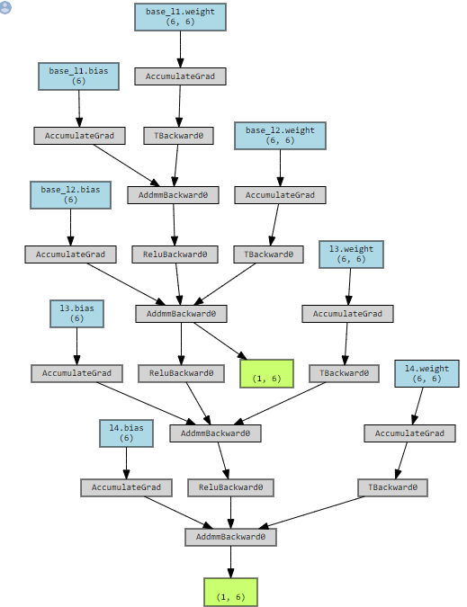
I could also join the gradient graph of this model you could easily notice that l1_base and l2_base layers can be learned without any help from l3 and l4 and vice versa if we backpropagate separately from the green rectangles presenting y_pred2 (the lower one) and y_pred1 (the upper one)
This “trick” won’t work as you are breaking the computation graph:
    # a trick to avoid the RuntimeError: Trying to backward through the graph a second
    # time ...
    y_pred1 = torch.tensor(y_pred1, requires_grad=True)
    loss1 = Loss(y_pred1, Y)
    l1.append(loss1)
    loss1.backward()
    optimizer1.step()
The RuntimeError is real and you could:
accumulate the losses and call backward() once
call backward() on each loss separately and then optimizer.step()
use backward(retain_graph=True) in the first backward call and make sure the forward activations are not stale to compute the gradients for loss1. I would consider this use case an advanced method and would not recommend to use it unless you know exactly that you want this behavior.
In your current code snippet you re avoiding the RuntimeError by detaching y_pred1 from the computation graph by recreating a new tensor with requires_grad=True. While this won’t raise any errors, no gradients will be created in the model parameters since y_pred1 is a new leaf tensor without any gradient history.
thank you for your reply and explanation. In fact, I had to go through all this because I need to update the value of y_pred1 based on the parameters update of optimezer2.step before running loss1. All this without altering the computation graph of y_pred1. more concretely optimizer2.step() will update the l3 layer. a column of this layer I want to reinject to y_pred1 data and then calculate loss1 based on this new value but with the same gradient history. thus I cannot use the first and second alternatives that you proposed.
I am doing this:
       loss2.backward(retain_graph=True)
       optimizer2.step()
       y_pred1.data = model.l3.weight[0, :].data.unsqueeze(0) # I am trying this one
       l1.append(loss1)
       loss1.backward()
       optimizer1.step()
is this valid? am I assigning a new value to the tensor y_pred1 and preserving everything else about its gradient?
why should y_pred1 be freed when calling loss2.backward() when the gradient is not a function of neither y_pred1, base_l1 nor base_l2? if retaining the gradient graph is a pain that we must go through could we do this partially? only for a set of parameters and not for the whole model?
thank you
Using the .data attribute is not recommended, as Autograd won’t track this change.
Based on your description, it seems however as if that’s exactly your use case. I.e. you want to inject a custom value into the graph, which was not created in a differentiable way.
Given that, I would highly recommend to manually check the gradient calculation and make sure that the gradients are indeed calculated as expected.
I don’t know where this approach is coming from so could you explain it a bit more?
exactly! that is what I was trying to do! and as you mentioned a manual check of this operation is a must.
about the second part of the question I think now I can formulate it in a better way:
to avoid grpah_retain=True, especially for big size models, it is possible to run loss2.backward() only on a subset of the model’s leaves. I think this helps us avoid allocating memory for retain_grad & avoid the wasted effort of calculating their gradient and then setting them back to 0 with optimizer2.zero_grad().
Yes, you can use the inputs argument to loss.backward to specify which tensors should be used for the gradient computation. All other tensors will be ignored.