New approach
So what you did now looks way better. Now you are really using the feature extractor to get some information from the architecture and use it. (and not the whole architecture).
How you may have seen, there are still some problems.
In order to fix them we need to truly understand what is happening with ViT and what we want to do. (That is why I asked what you intended to do with this.)
If your approach is to simply use ViT and classify directly with it, then there is a simpler approach. If as you mentioned, you want to use the “image features” and feed them to another architecture, then we need to understand ViT.
- ViT as classifier for N classes
- Use “image features” and feed them to something else
ViT as classifier for N classes
Here there is not much to understand. We have our architecture and in the end there is a head that classifies the image into N classes. To change this we only need to change the head to meet our needs and fine-tune the model.
For the torchvision implementation of vit_b_16, we can access the head like this
import torchvision

model = torchvision.models.vit_b_16(pretrained=True)
print(model.heads)

# Output:
#Sequential(
#  (head): Linear(in_features=768, out_features=1000, bias=True)
#)
So if we wanted to change this it would be very straighforward.
With this simple code we get our model with the right amount of classes and we can fine-tune it to classify our specific dataset.
import torch
import torchvision

N_CLASSES = 2

model = torchvision.models.vit_b_16(pretrained=True)
model.heads.head = torch.nn.Linear(768, N_CLASSES)
Use “image features” and feed them to something else
If we want to do this approach, then we need to first understand ViT.
Understanding ViT
So these are the steps that we will look into:
- Making patches
- Flatten the patches
- Class token
- Positional Embedding
- Encoder
- Head
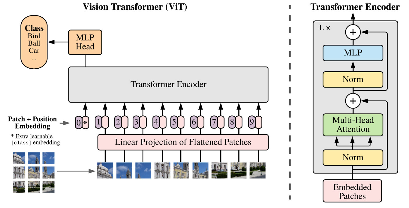
On the lower left corner of the image you can see how the image is divided into patches. For the architecture we are using (vit_b_16) each patch has 3x16x16 pixels. For an image with 224 pixels, we get 14x14 patches (14*16=224). This is why the input image has to have this size.
If we have a batch (B) of one image we could write it like this B x Patch_j x Patch_i x C x H x W = 1 x 14 x 14 x 3 x 16 x 16.
This means we have one image. This image has 14 patches in the y direction (j) and 14 patches in the x direction (i). Each of these patches have 3 channels. These patches also have 16 by 16 pixels in the x and y directions.
In the image above, we can see there is a pink box with the title Linear Projection of Flattened Patches. What we are making is rearanging these patches. So before we had this structure
B x Patch_j x Patch_i x C x H x W = 1 x 14 x 14 x 3 x 16 x 16
now we merge the 14x14 patches into one dimension. We also merge CxHxW into one direction.
B x Patches x Pixels = 1 x 14*14 x 3*16*16 = 1 x 196 x 768
This is also known as Batch x Seq_Length x Hidden_Dim.
So if we understand this, we can see that here the image has another meaning.
After this pink box on the architecture, there are several pink boxes with numbers and an extra box with an asterix on the left. As described on the image, this asterix is the Extra learnable [class] embedding. Here is where the results of the image transformer will be.
The size of this class token is B x 1 x Hidden_Dim = 1 x 1 x 768 for our case.
This is then prepended at the beggining of our representation of the image on the Seq_Length dim.
[cls]; img -> B x Seq_length + 1 x Hidden_Dim = 1 x 197 x 768.
Now Seq_length = 197. Here we have our 14x14 patches plus one for our [cls] token.
Also on the image we can see that a positional embedding is added. This is in order to see how the position of the patches relate to eachother.
The Dimentions however, stay the same.
B x Seq_Length x Hidden_Dim = 1 x 197 x 768
Now come the fun part. On the right of the image is the architecture of ONE encoder block. There are L blocks in the ViT architecture. (L=12 in ours). Meaning the image is fed to the first encoder block and the output of the first comes to the second and third sequentially.
All of the blocks have the same architecture, meaning the size of the output has to be the same as input in order to be fed to the next block.
Size_in = B x Seq_Length x Hidden_Dim = 1 x 197 x 768
Size_out = B x Seq_Length x Hidden_Dim = 1 x 197 x 768
If we look at how the block architecture is built, we can see some skip layers, batch normalizations and a multi-layer perceptron (MLP) in the end. There is also a Multi-Head Attention Layer (MHA).
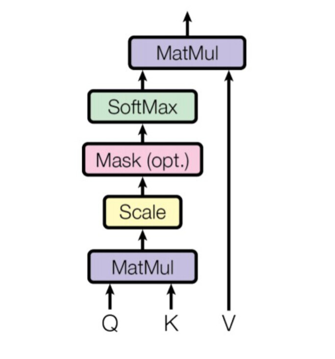
The MHA consists of multiple parallel scaled dot product attention mechanisms with learnable parameters.
One Scaled dot product attention looks like this
Described by the following equation
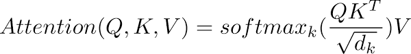
There is too much to unpack about this equation, but the important thing is that the pixels are attending to themselves. And HERE might be a good place to get the image features from.
To see how, see below in the Image Features section.
Up until now our data has the following format
B x CLS_Token+Seq_Length x Hidden_dim = 1 x 197 x 768.
We said that the CLS Token is where the classification will be done. So now we only take the CLS token and do not care for the rest.
B x CLS_Token x Seq_Length = 1 x 1 x 768
As we saw on the beggining of this post, the head consists (in this case) of a Linear layer that has 768 in features and 1000 features. This means that we feed our data to this Linear layer and we classify between 1000 classes.
On the image with the ViT architecture, this is represented by the yellow box with MLP Head written on it.
Image Features
Here is an implementation of tensorflow to get the attention map.
Here is a video + code on how to get them for pytorch.
Here is also a paper that might interest you.
These methods however, require that you either switch to TF or rewrite the ViT to access the attention map.
With feature extractor you can get intermediate steps (as we have already done by taking the getitem_5, which is almost the last step in the architecture).
If we inspect the graph_node_names as we did before to get the getitem_5 name, we can see that there is a encoder.layers.encoder_layer_11.self_attention. But the result is after doing the full Multi-Head Self-Attention.
We want an intermediate result.
So for this approach you could do something like this. (I ran this in a python notebook to see all of the heads.)
import matplotlib.pyplot as plt
import seaborn as sns
from PIL import Image
import requests
from io import BytesIO
import torchvision.transforms as T
from torchvision.models.feature_extraction import create_feature_extractor, get_graph_node_names
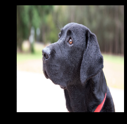
url = "https://www.thesprucepets.com/thmb/k3NXIqobAKvxoQ2ozGcwPxzIkpI=/3300x1856/smart/filters:no_upscale()/most-obedient-dog-breeds-4796922-hero-4440a0ccec0e42c98c5e58821fc9f165.jpg"
response = requests.get(url)
img = Image.open(BytesIO(response.content))
img = T.Resize((224,224))(T.ToTensor()(img))
plt.imshow(img.permute(1, 2, 0))
plt.show()
model = torchvision.models.vit_b_16(pretrained=True)
keys = ['encoder.layers.encoder_layer_11.ln']
feature_extractor = create_feature_extractor(model, return_nodes=keys)
feature_extractor.eval()
out = feature_extractor(img.unsqueeze(0))
x = out[keys[0]]
x_, attn = model.encoder.layers[-1].self_attention(x, x, x, need_weights=True, average_attn_weights=False)
print(x_.shape)
print(attn.shape)
for i in range(12):
sns.heatmap(attn[0, i, 0, 1:].view(14, 14).detach().numpy())
plt.show()
The output will be the 12 self attention heads ploted as heatmaps. As you will see, for this particular example, many will mean nothing to you but one of the heads looks like this.

If you set average_attn_weigths=True you will get the average of all 12 attention heads and will also mean nothing to us.
But if you also get the ‘heads’ key and print the predicted class, you will see that the predicted class is correct (208=Labrador retriever). So it means that it is working.
keys = ['encoder.layers.encoder_layer_11.ln', 'heads']
print(out['heads'].argmax(dim=1))
You could do something like this and use this self attention given by the ViT, but you need to understand what is happening and what you want to use and how.
Also, this will only be a suggestion of where important features might be. But these alone may mean nothing when feeding them to another architecture. So you might want to expriment by scaling them to the actual size of the image and feed both the image AND this heatmap to another architecture.
But these are just suggestions of what you could theretically do.
The most important thing is understanding what it does and how it does it. Then you can decide how to proceede with this information.
Hope this is a bit clearer now.