Hello everyone,
I am currently working on reinforcement learning experiments using a neural network and a differentiable physics simulator. My goal is to analyze the effects of different gradient modification methods on the training process. To implement these modifications, I need to perform both modified and original forward and backward passes using PyTorch.
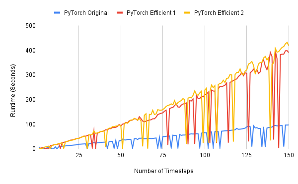
To improve efficiency, I attempted to replace two separate forward-backward passes with a single forward pass, followed by computing both original and modified gradients using loops over the computational graph. Theoretically, this should be more efficient, as it reduces redundant computations. However, in practice, I observed that these “efficient” implementations take more time than the original version, likely due to PyTorch’s optimized backward pass.
Additionally, as seen in the attached graph, the runtime does not always increase monotonically. Instead, at certain timesteps, there are sharp drops in runtime for both the original and modified implementations. Interestingly, when the “efficient” implementation experiences a drop, it actually becomes faster than the original version.
I have a few questions:
- What could be causing these sudden runtime drops in the backward pass?
- Are there any high-level (PyTorch API) or low-level (CUDA, autograd internals) optimizations that could help achieve these drops consistently?
- Would restructuring my computation graph or using different autograd functions improve efficiency in this case?
I would really appreciate insights from anyone with experience in PyTorch autograd internals or computational graph optimizations. Thank you in advance for your time and help!
(Attached: Graph illustrating the runtime behavior of different implementations averaged over 20 runs. Efficient 1 and Efficient 2 are 2 different versions for efficient computation graph.)