Hi pytorch friends!
I want to optimize per-example gradient computation, and found an interesting behavior when increasing the batch size. My findings can be reproduced in this notebook. Essentially I compute per-example losses then to call backward on each one:
t0 = time()
losses = loss_fn(model(samples), labels)
model.zero_grad()
for i, l in enumerate(losses):
    l.backward(retain_graph=True)
    # do something with the individual gradients
sampling_rate = batch_size / (time() - t0)
print(f"{sampling_rate:.0f} Hz")
I find that the computed sampling rate has a maximum for 20 to 60 samples dependent on the used GPU.
How can you (a) explain this behavior, and (b) possibly fix it so that I can get the most of my computations?
Thanks for considering my problem, please AMA
This is most likely because of the large number of calls to .backward().
Out of curiosity, how do you “# do something with the individual gradients” given that you don’t zero_grad() before? You do something with all the gradients accumulated up to now?
interesting; what type of overhead is generated by multiple calls to backward? Regarding curiosity, I omitted most of that (including zero_grad). It’s related to differential privacy.
What type of overhead does multiple calls to backward generate?
We need to go in cpp, discover the work that needs to be done, start GPU kernels for everything.
That takes some time.
omitted most of that (including zero_grad ). It’s related to differential privacy.
One thing I would say is that if the final transformation that you’re doing on the gradient is linear, then you can apply that same (similar) transformation to the loss before accumulation.
Otherwise, you can try to use something like this to get a per-sample gradients in one backward pass (more or less) and then do all the post processing after that. That might be faster.
I modified the code like so to investigate your explanantion:
for i, l in enumerate(losses):
    t = time()
    # just to do something with the gradients
    model.zero_grad()
    l.backward(retain_graph=True)
    print(i, time() - t)
Why do you think does it take four times as long to go to cpp in iteration 37 compared with iteration 36?
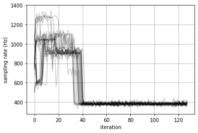
Here’s an infographics over a bunch of runs on my dedicated nv 2080 (sampling rate ~ 1 / (time() - t), iteration: that’s the index into the batch in the loop across losses):
However, thanks for the pointer to autograd hacks; I’ll try that out.
I would bet on you having filled the GPU task queue and so you now have to wait for stuff to be finished on the GPU before queuing more work.
The GPU api is asynchronous, so here, you only meansure the time to launch the jobs.
You can add torch.cuda.synchronize() before your timing if you want to measure the time it actually takes to compute the result.
That’s a great idea. I added that to the linked notebook (not saving it; you’ll have to do it yourself), and now I receive the following numbers on an nvidia T4:
at 3-batches, the sample rate is 614 +/- 122 Hz
at 24-batches, the sample rate is 883 +/- 132 Hz
at 64-batches, the sample rate is 380 +/- 5 Hz
at 96-batches, the sample rate is 265 +/- 2 Hz
I’m still a bit puzzled, though, that we observe a maximum sample processing rate at some 20 samples per batch. Wouldn’t one expect the runtime of the for-loop to scale linearly with the batch size, thus giving a nearly constant sample rate?
That is indeed interesting.
I did a quick test and it has nothing to do with the backwards: if you only measure the forward time, you see the same behavior
So I would guess that the kernel for larger batch size are more optimized than the ones for small batch size. And this is why you see this.
Note that if you use cudnn, it might even take completely different algorithms depending on the input shape!
Yeah, though I think it’s the other way around when trying to backprop sample-by-sample. Maybe it’s possible to somehow fix the algorithm to the version for small batch sizes.
I followed your advise, but to make it work for my GAN application I had to make some major adoptions of the code. I include this link here for other people’s reference that might encounter the same problem. Thanks again:
Also this is a modified version of your code that prints runtime instead of throughput. https://colab.research.google.com/drive/1aMCMZaSBak0PssL8nt2ff3mgFRKeNWaP
This makes it clear what happens: for small enough batch size, you get a sub-linear scaling as the GPU is under-utilized. At some point, you fully use the GPU and you start scaling linearly.
That would explain why the throughput looks this way.
@jusjusjus glad to see it was useful! I had a similar issue with GANs – saving forward quantities as module attribute means generator/discriminator passes got mixed together. Also, keeping activations around took too much memory, so I ended up using lower level autograd-lib for my application. Instead of storing activations in global variable, store them in closure-local variable, this way the memory gets released as you are done with the layer – example
The slowness has to do with batch size not saturating GPU compute units, so it could be called a hardware issue. However, autograd-hacks just restructures the computation to do a single large matmul instead of concatting together a bunch of small matmuls. Why couldn’t this be done automatically? In this sense it’s a software issue.
Are you sure about that? In a linear scaling, one expects what I call sample rate above (batch_size / (t1-t0)) to saturate. However, it starts to decrease with increasing batch sizes (see post above). Larger batches, it seems, are computed less efficiently than running multiple computes on smaller batches.
But the fact that you do as many backwards as there are samples in the batch makes them slower when the batch size increases.
In that case, I can buy that there is a sweet spot for a small number of samples.
Also note that each call to backward uses the FULL graph. So the more sample, the more expensive the backward for each individual sample.