I can’t figure out how to implement this operation with pytorch: \nabla \left( \nabla V_{\theta}^{\top}(s) \cdot \eta \right)

V_{\theta} is an ANN that takes in a vector ‘s’, the gradient is the partial w.r.t. weights of the NN and \eta is a the same size as the network weights.
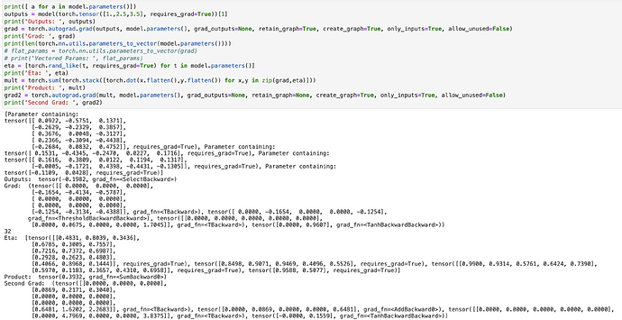
My main question: how to perform the second derivative in pytorch after taking the dot product with ‘\eta’?
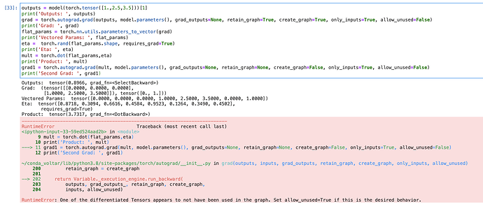
I am using autograd.grad(out,in), with in= ANN weights, and the out is the output for some ‘s’. This provides me with the first gradient. But then once I dot the first derivative with ‘\eta’, I am no longer able to computer the gradient with autograd.grad() because there is no computational graph.
# -*- coding: utf-8 -*-
import torch
import math


dtype = torch.float
device = torch.device("cpu")


# N is batch size; D_in is input dimension;
# H is hidden dimension; D_out is output dimension.
N, D_in, H, D_out = 64, 3, 5, 2

# Create random Tensors to hold inputs and outputs
x = torch.randn(N, D_in, device=device)
y = torch.randn(N, D_out, device=device)

# Use the nn package to define our model as a sequence of layers. nn.Sequential
# is a Module which contains other Modules, and applies them in sequence to
# produce its output. Each Linear Module computes output from input using a
# linear function, and holds internal Tensors for its weight and bias.
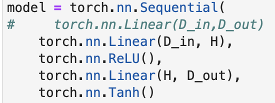
model = torch.nn.Sequential(
    torch.nn.Linear(D_in,D_out)
#     torch.nn.Linear(D_in, H),
#     torch.nn.ReLU(),
#     torch.nn.Linear(H, D_out),
)
model.to(device)
# The nn package also contains definitions of popular loss functions; in this
# case we will use Mean Squared Error (MSE) as our loss function.
loss_fn = torch.nn.MSELoss(reduction='sum')

learning_rate = 1e-4
for t in range(100):
    # Forward pass: compute predicted y by passing x to the model. Module objects
    # override the __call__ operator so you can call them like functions. When
    # doing so you pass a Tensor of input data to the Module and it produces
    # a Tensor of output data.
    y_pred = model(x)

    # Compute and print loss. We pass Tensors containing the predicted and true
    # values of y, and the loss function returns a Tensor containing the
    # loss.
    loss = loss_fn(y_pred, y)
    if t % 100 == 99:
        print(t, loss.item())

    # Zero the gradients before running the backward pass.
    model.zero_grad()

    # Backward pass: compute gradient of the loss with respect to all the learnable
    # parameters of the model. Internally, the parameters of each Module are stored
    # in Tensors with requires_grad=True, so this call will compute gradients for
    # all learnable parameters in the model.
    loss.backward()
    print(loss)

    # Update the weights using gradient descent. Each parameter is a Tensor, so
    # we can access its gradients like we did before.
    with torch.no_grad():
        for param in model.parameters():
            param -= learning_rate * param.grad


outputs = model(torch.tensor([1.,2.5,3.5]))[1]
grad = torch.autograd.grad(outputs, model.parameters(), grad_outputs=None, retain_graph=None, create_graph=False, only_inputs=True, allow_unused=False)
print([x.shape for x in grad])
eta =  [torch.rand(x.shape) for x in grad]
print(eta)
mult = sum([torch.dot(torch.flatten(x),torch.flatten(y)) for x,y in zip(grad,eta)])
mult.requires_grad = True
grad1 = torch.autograd.grad(mult, model.parameters(), grad_outputs=None, retain_graph=None, create_graph=False, only_inputs=True, allow_unused=False)


