print("CUDA available: ", torch.cuda.is_available())
device = torch.device("cuda" if torch.cuda.is_available() else "cpu")
CUDA available: True
x = torch.tensor([1, 2, 3]).to(device)
y = torch.tensor([1, 2, 3])
%%timeit -n 10000
z = x + 1
10000 loops, best of 3: 15.6 µs per loop
%%timeit -n 10000
z = y + 1
10000 loops, best of 3: 5.19 µs per loop
Note that CUDA operations are asynchronously executed, so you would need to time the operations in a manual loop and use torch.cuda.synchronize() before starting and stopping the timer.
Also, the workload is tiny, thus the kernel launch times might even be larger than the actual execution time.
do you mean something like this?
torch.cuda.synchronize(device=device) # before starting the timer

begin = time.time()

for i in range(1000000):

  z = x + 1

torch.cuda.synchronize(device=device) # before ending the timer

end = time.time()

total = (end - begin)/1000000; total
1.4210415363311767e-05
begin = time.time()

for i in range(1000000):

  z = y + 1

end = time.time()

total = (end - begin)/1000000; total
5.057124853134155e-06
still GPU takes longer time, so should I carry broadcasting operations on CPU, when using relatively small shape tensors?
Like I said, it depends on the workload.
If you would like to use only 3 numbers and your tensor is already on the CPU, just use the CPU.
Here is a quick comparison:
def time_gpu(size, nb_iter):
    x = torch.randn(size).to('cuda')
    torch.cuda.synchronize() # before starting the timer
    begin = time.time()

    for i in range(nb_iter):
        z = x + 1

    torch.cuda.synchronize() # before ending the timer
    end = time.time()
    total = (end - begin)/nb_iter
    return total


def time_cpu(size, nb_iter):
    y = torch.randn(size)
    begin = time.time()
    for i in range(nb_iter):
        z = y + 1

    end = time.time()
    total = (end - begin)/nb_iter
    return total


sizes = [10**p for p in range(9)]

times_gpu = []
for size in sizes:
    times_gpu.append(time_gpu(size, 10000))

times_cpu = []
for size in sizes:
    times_cpu.append(time_cpu(size, 1000))


import numpy as np
import matplotlib.pyplot as plt

fig, axarr = plt.subplots(2, 1)

axarr[0].plot(np.log10(np.array(sizes)),
              np.array(times_gpu),
              label='gpu')
axarr[0].plot(np.log10(np.array(sizes)),
              np.array(times_cpu),
              label='cpu')
axarr[0].legend()
axarr[0].set_xlabel('log10(size)')
axarr[0].set_ylabel('time in seconds')

axarr[1].plot(np.log10(np.array(sizes)),
              np.log10(np.array(times_gpu)),
              label='gpu')
axarr[1].plot(np.log10(np.array(sizes)),
              np.log10(np.array(times_cpu)),
              label='cpu')
axarr[1].legend()
axarr[1].set_xlabel('log10(size)')
axarr[1].set_ylabel('log10(time)')
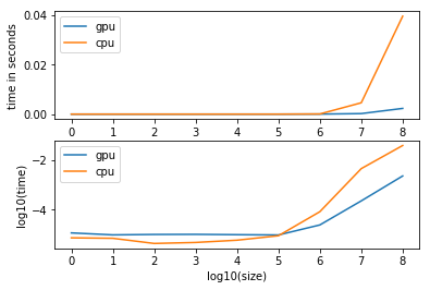
As you can see, the broadcast operation will have an approx. constant overhead up to a size of 10**5.
Using bigger tensors is a magnitude faster on the GPU.
1 Like