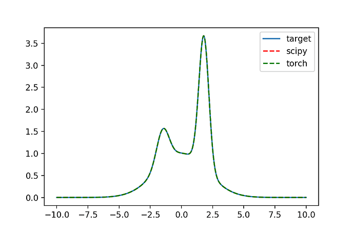
Preface: This question is not about training neural nets to perform curve fitting. I’m wondering about using the optimizers to perform minimization for curve fitting, with the aim of eventually moving calculations to the GPU.
Hi! I’m relatively new to using PyTorch. I’m wishing to use the pytorch’s optimizers with automatic differentiation in order to perform nonlinear least squares curve fitting. Since the Levenberg–Marquardt algorithm doesn’t appear to be implemented, I’ve used the L-BFGS optimizer. They both take advantage of second-order derivatives which PyTorch supports doing.
My question is how to improve the following code - in particular, I’m wondering about what I should be thinking about regarding the learning rate - the data fed to the optimizer is “smaller than memory” - somewhere between 2000 and 1 million data points.
import torch
from torch.functional import F

def gaussian(x, A=1, sigma=1, centre=0):
    return A*torch.exp(-(x - centre)**2 / (2*sigma**2))

def func(x, weights):
    'Takes a tensor of three sets of gaussian parameters, returns the sum of three gaussians'
    return gaussian(x, *weights[:3]) + gaussian(x, *weights[3:6]) + gaussian(x, *weights[6:9])

params = torch.tensor([0.8, 0.5, -1.5, 1, 2, 0, 3, 0.4, 1.8])
x = torch.linspace(-10, 10, 10000)
target = func(x, params)

guess = [1, 1, -0.2, 1, 1, 0.0, 1, 1, 0.2]
weights_LBFGS = torch.tensor(guess, requires_grad=True)
weights = weights_LBFGS

optimizer = torch.optim.LBFGS([weights_LBFGS], max_iter=10000, lr=0.1)
guesses = []
losses = []
def closure():
    optimizer.zero_grad()
    output = func(x, weights)
    loss = F.mse_loss(output, target)
    loss.backward()
    guesses.append(weights.clone())
    losses.append(loss.clone())
    return loss

%time optimizer.step(closure) # %time is jupyter timing magic - remove it to run this outside ipython
print(f"Minimum: {[v.item() for v in weights]}")
print(f"Number of steps: {len(guesses)}")

# Wall time: 683 ms
# Minimum: [0.8001920580863953, 0.4998912513256073, -1.4998143911361694, 0.9999790787696838, 2.0001237392425537, 0.00012422756117302924, 2.9998154640197754, 0.4000047743320465, 1.7999995946884155]
# Number of steps: 256
The fit works, but it takes time - about ten times what scipy does using scipy.optimize.curve_fit. If I move it onto the GPU (by adding device='cuda' to the tensor functions), it takes a further 10 times as long! (5 sec)
import numpy as np
from scipy.optimize import curve_fit

def gaussian_numpy(x, A=1, sigma=1, centre=0):
    return A*np.exp(-(x - centre)**2 / (2*sigma**2))

def func_numpy(x, *weights):
    return gaussian_numpy(x, *weights[:3]) + gaussian_numpy(x, *weights[3:6]) + gaussian_numpy(x, *weights[6:9])

xi = x.numpy()
yi = target.numpy()

%time fit, err = curve_fit(func_numpy, xi, yi, p0=guess, method='lm')
Both cases produce a good fit, but I would need to improve the speed before I can consider using it as an alternative to scipy. I have played with some other optimizers (Adam) but it seems to perform rather poorly for this - I can go more into detail on that in a reply below.
# Visualising the fit
import matplotlib.pyplot as plt
plt.figure(dpi=150)
plt.plot(xi, yi, label='target')
plt.plot(xi, func_numpy(xi, *fit), ls='--', color='red', label='scipy')
plt.plot(xi, func(x, weights_LBFGS).detach(), ls='--', color='green', label='torch')
plt.legend()
