What does tensor.backward(..) do mathematically?

[maaft]

I have very hard times, understanding what tensor.backward(…) does in mathematical terms.

Assuming we have a pre-trained model and doing a forward pass.
model.zero_grad()
y = model(x)

Afterwards, we do a backward step on the output using the ground-truth target.
y.backward(gradient=target)

What is exactly happening here in mathematical terms? What is the gradient argument supposed to be and why is the ground-truth target often used here?

After doing the backward step, what result will I have in x.grad (mathematically)?

Is x.grad different from getting the gradient via register_backward_hook on the first layer?
If yes, what result (mathematically) did I “hook” instead of x.grad ?

    def hook_layers(self):
        def hook_function(module, grad_in, grad_out):
            self.gradients.append(grad_in[0])


        # Register hook to the first layer

        self.model.conv1.register_backward_hook(hook_function)

I hope this makes sense. If you need clarifications, please feel free to ask!

[albanD]

Hi,

If y is of size N, then y.backward(gradient) will use the chain rule to compute the gradient for every parameter in the network. For a give param, w of size d, it will perform: gradient * dy/dw where dy/dw will will be computed by the chain rule.

If loss is a tensor with a single element, loss.backward() is the same as loss.backward(torch.Tensor([1])) and thus will compute for every parameter w: 1 * dloss / dw = dloss / dw. And so the .grad attribute of each w will just contain this gradient.

I am not sure where you saw people doing y.backward(gradient=target) but that basically corresponds to having a loss function loss = sum(y * target). Because 1 * dloss / dy * dy / dw = target * dy / dw because given the loss definition above dloss / dy = target. I don’t know where such loss function is used though.

Warning: register_backward_hook is kinda broken at the moment for nn.Modules and you should avoid relying on them.
But it should give you extactly the same thing as input.grad.

Also note that the .grad field is populated only for leaf tensors (that you created with requires_grad=True) or tensors for which you explicitly called retain_grad=True.

[maaft]

Thanks for your reply.

Setting the target class for gradient= is used when visualizing what the model does w.r.t. to given input image. (To see what the model focusses on when classifying objects)
See https://github.com/utkuozbulak/pytorch-cnn-visualizations#gradient-visualization.

As I am not doing classification but rather regression, I tried to modify the above source code.
Given an input image, my model should predict the pixelwise scene-depth (i.e. distance to the camera in meters). Now, I want to visualize what features my model thinks are important for doing depth prediction.

General question: Is it correct to assume that a big dy/dx (i.e. big x.grad) for a particular pixel means that the model pays more attention to that pixel?

After following your derivations, I think that setting gradient= to my ground-truth depth does not make any sense at all. This would only introduce a weighting factor that prefers pixels which are further away from the camera (but could potentially be still very important for the overall depth prediction). I think it would make more sense to just set gradient= to torch.ones(target.shape).

Is it possible to use LaTeX math markdown or similar? This plain-text math is awful to read!

I can’t follow your derivation: loss = sum(y * target) , dloss / dy = target. I think it should rather equate to dloss / dy = sum(target). And therefore: dloss / dy * dy / dw = sum(target) * dy / dw.

Anyway, I think your introduction of an equivalent loss function really confuses me.

[albanD]

In your case passing either a tensor of all ones will let you know how sensitive is the sum of the output wrt each input pixel.
If you give a tensor of zeros and a single one for one pixel, it will let you know how sensitive is the predicted depth value for that pixel wrt each input pixel.

Yes there is no math formatting unfortunately
dloss / dy = target is correct (I think), as loss is a number and y a tensor, dloss / dy should be a tensor of the same size as y, target in this case. The sum(target) is a number and cannot correspond to that gradient:
Assuming y and w being 1D tensors, your formulation dloss / dw = dloss / dy * dy / dw = sum(target) * dy / dw does not make sense as dloss / dw is 1 x w.size() but the last term is of size y.size() x w.size().

[mratsim (Mamy Ratsimbazafy)]

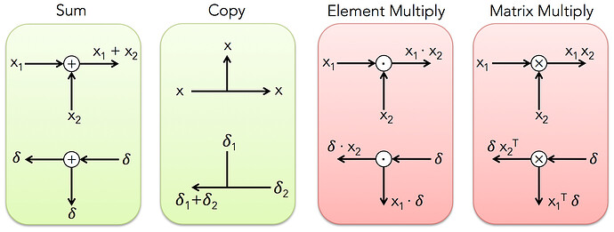
Backward is doing “reverse mode auto-differentiation” in mathematical terms.

You can follow this excellent tutorial by Andrej Karpathy to get an intuition of what is going on.

And this blog post from Baidu’s Silicon Valley AI Labs has very good figures as well.

Finally, here is my own implementation of a scalar autograd, it’s just 3 files, less than 500 lines and it’s in Nim which has a syntax similar to Python but with types. It should be pretty readable. The backward proc is just 30 lines.

The main difference with PyTorch implementation is that for this autograd I choose to return closures (i.e. function object) instead of saving state for the backward pass in an object with forward and backward method. spaCy backend “Thinc” is also implemented the same way.

To go a bit in the details with “sin” and “cos” example:

template bp_negate_sin[T](value: T): BackProp[T] =
  (gradient: T) => - gradient * value.sin()

template bp_cos[T](value: T): BackProp[T] =
  (gradient: T) => gradient * value.cos()

proc cos*[T](v: Variable[T]): Variable[T] =
  return Variable[T](
           tape: v.tape,
           value: v.value.cos(),
           index: v.tape.push_unary(v.index, bp_negate_sin(v.value))
           )

proc sin*[T](v: Variable[T]): Variable[T] =
  return Variable[T](
           tape: v.tape,
           value: v.value.sin(),
           index: v.tape.push_unary(v.index, bp_cos(v.value))
           )

I have a tape that records all operations during the forward pass. A value field that has the current value and an index of the operation in the tape. backward then just unwind the tape and call bp_cos (backprop_cos) when it finds its index.

Let’s take a binary operation now like -

proc bp_identity[T](gradient: T): T = gradient
proc bp_negate[T](gradient: T): T = -gradient

proc `-`*[T](lhs: Variable[T], rhs: Variable[T]): Variable[T] =
  return Variable[T](
           tape: lhs.tape,
           value: lhs.value - rhs.value,
           index: lhs.tape.push_binary(
             lhs.index, bp_identity[T],
             rhs.index, bp_negate[T]
             )
           )

In the tape I keep track of both the left-hand side and right-hand side operand which are respectively identity and negate.

[maaft]

Thanks again! Of course, you were right with your derivation. I somehow applied scalar derivation rules for vectors which is of course wrong. My bad, sorry.

@albanD

In your case passing either a tensor of all ones will let you know how sensitive is the sum of the output wrt each input pixel.

In other words: A pixel with high dy/dx contributes a lot to the final network output. Correct? So when visualizing x.grad I will obtain an “attention” map of the input image.

Input Image ------------------------------------------------- dsum(y)/dx (i.e. x.grad after y.backward(torch.ones(…)))

Therefore, looking at these images, I can say that the network pays attention to edges (surprise!). Any idea what that wiggly stuff could relate to? Maybe some texture-filters?

[albanD]

Not sure the wiggly stuff are but it is interesting to see that they are color dependant. While most things are grey here, they actually give different values for different color channels.

Also Setting a 1 for only a single pixel might tell you which input would affect it’s value. Giving you informations about how far from the pixel it looks.