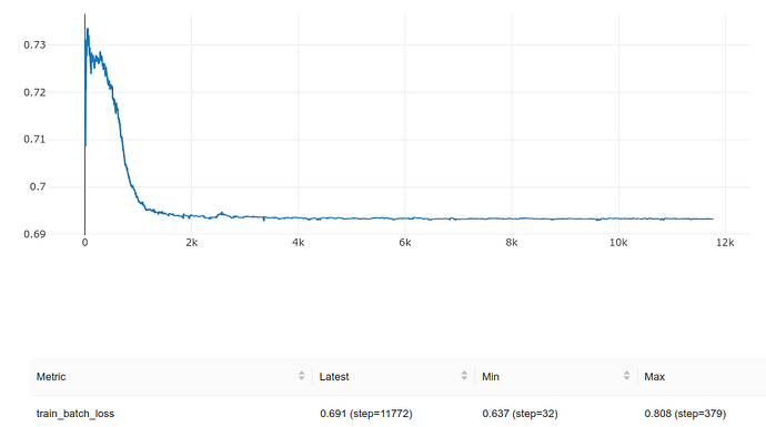
BCE loss stuck at 0.693 in the beginnng of training and then started to decrease, why?

Cyber_punk · July 11, 2023, 12:24pm

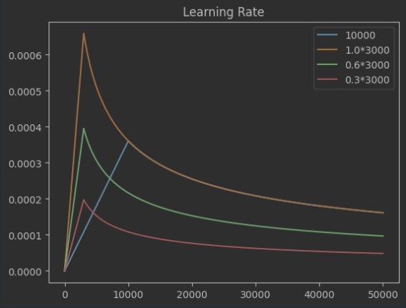
I’m using a Transformer encoder with a binary cross entropy loss for CTR prediction. The training batch loss is at around 0.693 constantly for the beginning several thousand steps (batches). I’m using Noam learning rate schedule and a scaling factor for setting the learning rate used by Adam. The first 3000 steps are the warm up steps in Noam:

lr= factor * ( model_size ** (-0.5) * min(step** (-0.5), step *
warmup_steps ** (-1.5)) )

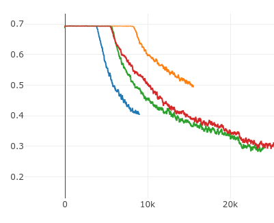
For the learning rate, when setting scaling factor to be 0.5 or 0.6, the period with constant 0.693 is from beginning to 5500th steps. When I use lower lr by setting scaling factor 0.3, the period with constant 0.693 became longer (8000 steps). When I use higher lr by setting scaling factor 1.0, the period with constant 0.693 became shorter (4000 steps).

Note: the above training batch loss curve is smoothed.

Does this mean I should use a high learning rate (e.g., with scale factor being 1.0)?
Why there is a period with constant 0.693 loss? is it because the learning rate is too small to make any adjustment to the parameters? If so, after the 3000 warmup steps the learning rate is even smaller, why the loss is decreasing?

KFrank · July 11, 2023, 4:39pm

Hi Cyber!

Note that log (1/2) = -0.693147, which is the same as
torch.nn.functional.logsigmoid (torch.tensor (0.0)).

This is telling us that your model is predicting values that are zero (or
that are tightly clustered around zero). Look at the values your model
is predicting during its “constant period.”

How are you initializing the weights of your model? You typically want
to initialize your weights randomly so that you don’t get stuck in some
“symmetric” configuration (that, perhaps, predicts zeros). If you are
using random initialization, you might want to try increasing the scale
(typical size or standard deviation) of those random weights. Pay
particular attention to the last few layers of your model. Does your
output layer have a bias?

Do you have ReLUs or other activations that could be starting off
“saturated” at or near zero, especially near the end of your model?

(Using a higher learning rate could certainly get you out of your
“constant period” faster, but it would seem to be a better approach
not to start out in a predict-zero phase in the first place.)

Best.

K. Frank

Cyber_punk · July 12, 2023, 7:06am

Thanks for your informative analysis!

The input layers are embedding layers initialized with uniform(-0.1, 0.1):

init_range = 0.1
self.job_id_embedding_layer.weight.data.uniform_(-init_range, init_range)

The intermediate layers are a Transformer encoder block. I didn’t change the initialization methods for the weights.

The last few layers are a 3-layer FFNN block:

self.linear = nn.Sequential(
    nn.Linear(768 * 2, 1024),
    nn.LeakyReLU(),
    # nn.LayerNorm(1024),
    nn.Linear(1024, 512),
    nn.LeakyReLU(),
    # nn.LayerNorm(512),
    nn.Linear(512, 256),
    nn.LeakyReLU(),
    # nn.LayerNorm(256),  # Layer norm
    nn.Linear(256, 1)
)
logits = self.linear(features.view(features.size()[0], -1))

I’m using the default initialization method for the linear layers as well. It looks it’s Xavier initialization:

weight – the learnable weights of the module of shape (out_features, in_features). The values are initialized from U( − √(k), √(k)), where k = (1)/( in_features)
bias – the learnable bias of the module of shape (out_features). If bias is True, the values are initialized from U( − √(k), √(k)) where k = (1)/( in_features)
The nn.Linear layers have bias by default. Is it better to not have biases for these linear layers?
I’m using LeakyReLU activation function for these last few linear layers.

From your comment,
(1) weight initialization for layers especially the last few layers:
Increasing the scale (typical size or standard deviation) of those random weights

(2) bias?

(3) ReLU:
Avoid ReLU because it’s easy to get “turned off” by becoming 0?

Also, Would using nn.LayerNorm in the last few layers be helpful in solving the constant 0.693 loss problem? I wasn’t using them in my last run.

Update regarding using LayerNorm: adding LayerNorm after the last few linear layers with leakyReLU actually made it worse - the loss stuck at 0.693 forever:

KFrank · July 12, 2023, 4:09pm

Hi Cyber!

If I understand you correctly, the very last layer of your model is
Linear (256, 1).

I assume that you then pass logits to BCEWithLogitsLoss()

(As an aside, if you’re using BCELoss, you should instead be using
BCEWithLogitsLoss. However, my main comment about the constant
loss would still be true, but just with your input being 0.5 instead of
0.0.)

Look at the values you get for logits right at the beginning and early on
in the training. How close are they to zero?

Also, print out your loss to full precision (e.g., print (loss.item()). How
close is your loss to being exactly log (2)?

With default weight initialization, your weights should be large enough
that your logits should be enough different than 0.0 that your loss
should not be almost exactly log (2).

Consider:

>>> import torch
>>> torch.__version__
'2.0.0'
>>> _ = torch.manual_seed (2023)
>>> lin = torch.nn.Linear (256, 1)   # your last layer
>>> lin.bias   # not that close to zero
Parameter containing:
tensor([0.0269], requires_grad=True)
>>> logits = lin (torch.zeros (256))
>>> logits   # not zero even though the input to lin is zero
tensor([0.0269], grad_fn=<AddBackward0>)
>>> torch.nn.BCEWithLogitsLoss() (logits, torch.ones (1))   # not that close to log (2)
tensor(0.6798, grad_fn=<BinaryCrossEntropyWithLogitsBackward0>)
>>> torch.nn.BCEWithLogitsLoss() (torch.zeros (1), torch.ones (1))   # input of zero gives log (2)
tensor(0.6931)

In general, you do want to use bias in your Linear layers (and
convolutions, for that matter).

In general, ReLU is a satisfactory activation. It can get “stuck” in its
“turned off” regime, but this tends not to be a problem in practice.

In any event, you are using LeakyReLU, which avoids this problem.

As far as this particular problem goes, LayerNorm is irrelevant. As noted
above, your final layer has non-zero bias, so the logits you output won’t
be zero.

To track this down, check the actual logits output by your model. Check
the actual predicted values you input to your loss function. Print out the
bias of your last layer (your Linear (256, 1)) before you start training.
Plot the deviation of your loss from log (2) as you train.

Please also post the part of your code where you instantiate your loss
criterion and where you pass your predictions to your loss criterion.

Best.

K. Frank

dhruvbird · July 12, 2023, 5:50pm

@ Cyber_punk Do you have a data imbalance in your labels? For example, maybe you have a lot more samples with no click than with click. That may also affect how quickly the model can start learning. In practice however, I’ve seen that models tends to learn to predict the overrepresented class pretty quickly though, so maybe you have a deep network or a very low learning rate (or both), which can exacerbate things.

Cyber_punk · July 13, 2023, 9:26am

Hi K. Frank,
Yes, the last layer is nn.Linear(256, 1), and the logits are passed to BCEWithLogitsLoss().

I did a few runs and for about (sometimes before and sometimes after) 5000 steps the train batch loss was fluctruating around 0.693.

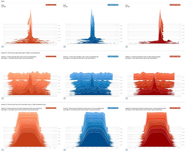
The distribution of logits in batches of 64 samples are indeed very close to 0s during these 5000 steps. It was very “narrow” distribution centered around 0. But after the initial 5000 steps, the distribution of logits started to be scattered around in a relatively larger scale. The following is for 3 runs:

During these initial 5000 steps, the BCE loss is very close to 0.693 or log(2):

run_id,key,value,step,timestamp
390b7bed44bc4cb39c5c55cfed6cbcde,train_batch_loss,0.6891335844993591,1,1689070859610
390b7bed44bc4cb39c5c55cfed6cbcde,train_batch_loss,0.6845006346702576,2,1689070859728
390b7bed44bc4cb39c5c55cfed6cbcde,train_batch_loss,0.6913905143737793,3,1689070859858
390b7bed44bc4cb39c5c55cfed6cbcde,train_batch_loss,0.693462610244751,4,1689070859981
390b7bed44bc4cb39c5c55cfed6cbcde,train_batch_loss,0.6899896264076233,5,1689070860125
390b7bed44bc4cb39c5c55cfed6cbcde,train_batch_loss,0.697765588760376,6,1689070860260
390b7bed44bc4cb39c5c55cfed6cbcde,train_batch_loss,0.7007498145103455,7,1689070860400
390b7bed44bc4cb39c5c55cfed6cbcde,train_batch_loss,0.7083665132522583,8,1689070860508
390b7bed44bc4cb39c5c55cfed6cbcde,train_batch_loss,0.6904076933860779,9,1689070860619
390b7bed44bc4cb39c5c55cfed6cbcde,train_batch_loss,0.6960662603378296,10,1689070860750
390b7bed44bc4cb39c5c55cfed6cbcde,train_batch_loss,0.7000266909599304,11,1689070860854
390b7bed44bc4cb39c5c55cfed6cbcde,train_batch_loss,0.6916379928588867,12,1689070860984
390b7bed44bc4cb39c5c55cfed6cbcde,train_batch_loss,0.7038472294807434,13,1689070861120
390b7bed44bc4cb39c5c55cfed6cbcde,train_batch_loss,0.695785403251648,14,1689070861232
390b7bed44bc4cb39c5c55cfed6cbcde,train_batch_loss,0.6908349990844727,15,1689070861331
...
...
390b7bed44bc4cb39c5c55cfed6cbcde,train_batch_loss,0.6938340663909912,5298,1689071557099
390b7bed44bc4cb39c5c55cfed6cbcde,train_batch_loss,0.6932273507118225,5299,1689071557211
390b7bed44bc4cb39c5c55cfed6cbcde,train_batch_loss,0.6899099946022034,5300,1689071557334
390b7bed44bc4cb39c5c55cfed6cbcde,train_batch_loss,0.6955896019935608,5301,1689071557467
390b7bed44bc4cb39c5c55cfed6cbcde,train_batch_loss,0.6937833428382874,5302,1689071557567
390b7bed44bc4cb39c5c55cfed6cbcde,train_batch_loss,0.6919088363647461,5303,1689071557679
390b7bed44bc4cb39c5c55cfed6cbcde,train_batch_loss,0.6920832395553589,5304,1689071557783
390b7bed44bc4cb39c5c55cfed6cbcde,train_batch_loss,0.6949018239974976,5305,1689071557898
390b7bed44bc4cb39c5c55cfed6cbcde,train_batch_loss,0.6921497583389282,5306,1689071558024

The bias of last layer (Linear (256, 1)) seems to be pulled towards 0 in the beginning 5000 steps, regardless of the initialized value being positive or negative:

I’ve also plotted the histgrams of the weights of the last and the second to the last linear layers. It looks the distribution of weight of the linear layers before the last linear layer didn’t change much during the first 5000 steps. If the distribution of weight does not change much, maybe the speicifc values are not changing much then.

The following is the part related to loss criterion. I used DDP for running the model, but actually I’m running it on my local PC with a single GPU.

self.ddp_model = DDP(model, device_ids=[gpu_id], find_unused_parameters=True)  # False
...
self.criterion = nn.BCEWithLogitsLoss(reduction='mean')  # batch loss mean
...

for train_batch in self.train_dataloader:

    train_batch_step += 1
    self.optimizer.zero_grad()
    output = self.ddp_model(**get_features(train_batch, self.gpu_id))
    train_batch_loss = self.criterion(output, get_label(train_batch, self.gpu_id))
    train_batch_loss.backward()
    self.optimizer.step()
    self.lr_scheduler.step()

Cyber_punk · July 13, 2023, 9:47am

Hi @dhruvbird , I think I don’t have data imbalance issue. The raw data only has positive class (clicks). I sampled the negative samples based on popularity with exactly 1:1 proportion.

After the negative sampling, I splitted the train and validation sets based on TimeSeriesSplit. The clicking data in validation set are always after the clicking behaviours in training data.

In training, I did shuffling on the training dataloader (shuffle is True by default for DistributedSampler):

    # Setting num_workers as 4 * num of GPUs
    train_dataloader = DataLoader(
        dataset_dict["train"], batch_size=batch_size, collate_fn=custom_collate_function, pin_memory=True,
        num_workers=num_workers,
        shuffle=False,
        sampler=DistributedSampler(dataset_dict["train"])
    )
    valid_dataloader = DataLoader(
        dataset_dict["valid"], batch_size=batch_size, collate_fn=custom_collate_function, pin_memory=True,
        num_workers=num_workers,
        shuffle=False,
        sampler=DistributedSampler(dataset_dict["valid"], shuffle=False, drop_last=True)  # 504114 % (64 * 4) == 50 samples
    )

I think the 0.693 loss issue probably has something to do with the last fully connectly block with 4 linear layers and leakyReLU layers as mentioned by KFrank. Because when I replaced the whole fully connectly block with an inner product operation, there is no more 0.693 loss issue. But there is another problem, so I posted it separately: Does my loss curve show the model is overfitting?

KFrank · July 14, 2023, 1:18am

Hi Cyber!

Okay, this makes good sense. The initial value and early values of your
loss are not “almost exactly” log (2), but an amount away that is
consistent with the size of the initial value of Linear (256, 1).bias,
which itself is more or less the value of the initial predicted logit.

Note that binary cross entropy penalizes your model more for guessing
wrong than it rewards it for guessing right, so if your model doesn’t (yet)
have a good prediction, it’s best off predicting a logit of zero (which
translates to a probability of one half – i.e., don’t know, so flip a coin).
So – until the rest of your model starts learning how to make a prediction
with some value to it – it makes sense for your final bias to get trained
down to zero.

As to why it takes seemingly so long to start training effectively, I don’t
really know.

If it were me, I would try increasing the initial learning rate until it starts
getting out of the “stuck” phase more expeditiously (or until the initial
training starts to become unstable and diverges).

It’s just me, but when training isn’t “behaving,” I generally like to start
with plain-vanilla SGD, using as large a learning rate as I can without
things diverging. Then I’ll back off on the learning rate a little, and start
turning on SGD’s momentum. (Sometimes you have to train for a
shortish warm-up period with a smaller learning so the parameters get
non-wacky before turning up the learning rate or momentum.)

Note, even if Adam ends up training more effectively than SGD, there
is nothing wrong with training with SGD to get out of the “stuck” phase
and then switching over to Adam.

Or, if the “stuck” phase doesn’t really matter in terms of computer time,
you can just stick with your current training scheme and view those first
5000 training iterations as the price of admission.

Best.

K. Frank

kappablanca · October 10, 2024, 2:24pm

I know it is an old post, but for anyone stumbling on this. What is happening here is that the weights of the final linear layer are driven to zero in the first few training steps. This is due to the fact that the transformer was not yet able to pick up on the pattern of the data and your final layer is minimizing the BCE loss by always predicting the mean of your data.

I had this problem myself and I fixed it by adding a loss term preventing the standard deviation to go to zero. I described this here: https://open.substack.com/pub/yannikkeller/p/solving-vanishing-gradients-from?r=3avwpj&utm_campaign=post&utm_medium=web