How to make CNN performance better, CNN accuracy cannot convergent

[Raden (raden renggala)]

hi everyone,
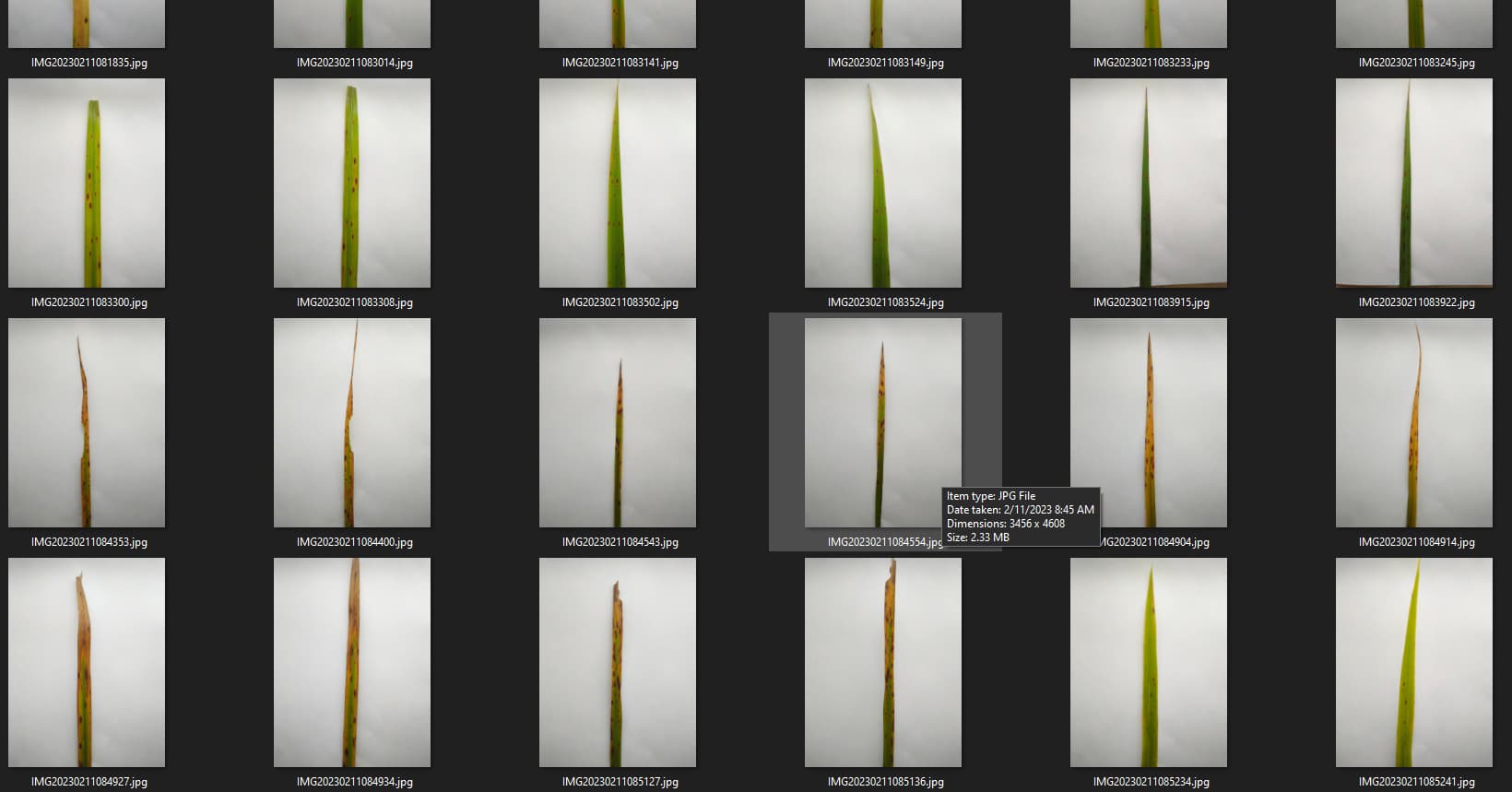
I just learned about CNN and I want to create a custom architecture to classify 2 classes of rice leaf disease (leaf blight and leaf spot), with a relatively small total data, namely 1080 data on rice leaf in a photo on a white background. training has been carried out several times but the accuracy is not convergent.
what should I do to achieve good results.

def DepthConvBlock(in_channels, out_channels, stride=1):
    return nn.Sequential(
        nn.Conv2d(in_channels, in_channels, kernel_size=3, stride=stride, padding=1, groups=in_channels),
        nn.BatchNorm2d(in_channels),
        nn.ReLU(inplace=True),
        nn.Conv2d(in_channels, out_channels, kernel_size=1, stride=1),
        nn.BatchNorm2d(out_channels),
        nn.ReLU(inplace=True)
    )

class CNNpenyakitPadi(nn.Module):
    def __init__(self, output_size):
        super().__init__()
        self.feature = nn.Sequential(

            DepthConvBlock(3, 16, stride=1),
            nn.MaxPool2d(2, 2),
            
            DepthConvBlock(16, 32, stride=1),
            nn.MaxPool2d(2, 2),
            
            DepthConvBlock(32, 64, stride=1),
            nn.MaxPool2d(2, 2),
            
            DepthConvBlock(64, 128, stride=1),
            nn.MaxPool2d(2, 2),
            
            DepthConvBlock(128, 256, stride=1),
            nn.MaxPool2d(2, 2),
            
            DepthConvBlock(256, 512, stride=1),
            nn.AdaptiveMaxPool2d(1)
            
        )
        self.classifier = nn.Sequential(
            nn.Linear(512, output_size),
            nn.Dropout(0.5)
        )

    def forward(self, x):
        x = self.feature(x)
        x = x.view(x.size(0), -1)
        x = self.classifier(x)
        return x

some of the settings used

device = torch.device("cuda" if torch.cuda.is_available() else "cpu")
model = CNNpenyakitPadi(output_size = len(train_set.classes)).to(device)
criterion = nn.CrossEntropyLoss()
optimizer = optim.AdamW(model.parameters(), lr=0.0015, weight_decay=0.005, amsgrad=False)
callback = Callback(model, early_stop_patience=10, outdir="modelC6")

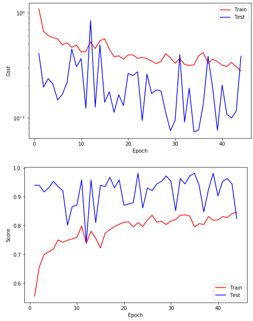
This is the result of training in several epochs

Epoch     1
Train_cost  = 1.0851 | Test_cost  = 0.4106 | Train_score = 0.5544 | Test_score = 0.9398 |

Epoch     2
Train_cost  = 0.6667 | Test_cost  = 0.1962 | Train_score = 0.6562 | Test_score = 0.9398 |

Epoch     3
Train_cost  = 0.6072 | Test_cost  = 0.2363 | Train_score = 0.6991 | Test_score = 0.9167 |
==> EarlyStop patience =  1 | Best test_cost: 0.1962

Epoch     4
Train_cost  = 0.5799 | Test_cost  = 0.2092 | Train_score = 0.7083 | Test_score = 0.9306 |
==> EarlyStop patience =  2 | Best test_cost: 0.1962

Epoch     5
Train_cost  = 0.5638 | Test_cost  = 0.1479 | Train_score = 0.7188 | Test_score = 0.9537 |

Epoch     6
Train_cost  = 0.4966 | Test_cost  = 0.1675 | Train_score = 0.7500 | Test_score = 0.9352 |
==> EarlyStop patience =  1 | Best test_cost: 0.1479

Epoch     7
Train_cost  = 0.5178 | Test_cost  = 0.2169 | Train_score = 0.7419 | Test_score = 0.9213 |
==> EarlyStop patience =  2 | Best test_cost: 0.1479

Epoch     8
Train_cost  = 0.4695 | Test_cost  = 0.4520 | Train_score = 0.7488 | Test_score = 0.8009 |
==> EarlyStop patience =  3 | Best test_cost: 0.1479

Epoch     9
Train_cost  = 0.4929 | Test_cost  = 0.3073 | Train_score = 0.7535 | Test_score = 0.8657 |
==> EarlyStop patience =  4 | Best test_cost: 0.1479

Epoch    10
Train_cost  = 0.4230 | Test_cost  = 0.3656 | Train_score = 0.7593 | Test_score = 0.8704 |
==> EarlyStop patience =  5 | Best test_cost: 0.1479

Epoch    11
Train_cost  = 0.4288 | Test_cost  = 0.1234 | Train_score = 0.7986 | Test_score = 0.9583 |

Epoch    12
Train_cost  = 0.5295 | Test_cost  = 0.8451 | Train_score = 0.7384 | Test_score = 0.7407 |
==> EarlyStop patience =  1 | Best test_cost: 0.1234

Epoch    13
Train_cost  = 0.4564 | Test_cost  = 0.1270 | Train_score = 0.7801 | Test_score = 0.9583 |
==> EarlyStop patience =  2 | Best test_cost: 0.1234

Epoch    14
Train_cost  = 0.5418 | Test_cost  = 0.4970 | Train_score = 0.7558 | Test_score = 0.8102 |
==> EarlyStop patience =  3 | Best test_cost: 0.1234

Epoch    15
Train_cost  = 0.5663 | Test_cost  = 0.1406 | Train_score = 0.7222 | Test_score = 0.9398 |
==> EarlyStop patience =  4 | Best test_cost: 0.1234

Epoch    16
Train_cost  = 0.4501 | Test_cost  = 0.1768 | Train_score = 0.7731 | Test_score = 0.9352 |
==> EarlyStop patience =  5 | Best test_cost: 0.1234

Epoch    17
Train_cost  = 0.3807 | Test_cost  = 0.1128 | Train_score = 0.7859 | Test_score = 0.9676 |

Epoch    18
Train_cost  = 0.3899 | Test_cost  = 0.1658 | Train_score = 0.7963 | Test_score = 0.9306 |
==> EarlyStop patience =  1 | Best test_cost: 0.1128

Epoch    19
Train_cost  = 0.3616 | Test_cost  = 0.1310 | Train_score = 0.8044 | Test_score = 0.9583 |
==> EarlyStop patience =  2 | Best test_cost: 0.1128

Epoch    20
Train_cost  = 0.3970 | Test_cost  = 0.2650 | Train_score = 0.8113 | Test_score = 0.8704 |
==> EarlyStop patience =  3 | Best test_cost: 0.1128


Epoch    21
Train_cost  = 0.3979 | Test_cost  = 0.2523 | Train_score = 0.8125 | Test_score = 0.8750 |
==> EarlyStop patience =  4 | Best test_cost: 0.1128

Epoch    22
Train_cost  = 0.3689 | Test_cost  = 0.2745 | Train_score = 0.7951 | Test_score = 0.8796 |
==> EarlyStop patience =  5 | Best test_cost: 0.1128

Epoch    23
Train_cost  = 0.3753 | Test_cost  = 0.0942 | Train_score = 0.8102 | Test_score = 0.9815 |

Epoch    24
Train_cost  = 0.3673 | Test_cost  = 0.2607 | Train_score = 0.7963 | Test_score = 0.8611 |
==> EarlyStop patience =  1 | Best test_cost: 0.0942


Epoch    25
Train_cost  = 0.3467 | Test_cost  = 0.1702 | Train_score = 0.8194 | Test_score = 0.9306 |
==> EarlyStop patience =  2 | Best test_cost: 0.0942

Epoch    26
Train_cost  = 0.3278 | Test_cost  = 0.1846 | Train_score = 0.8356 | Test_score = 0.9213 |
==> EarlyStop patience =  3 | Best test_cost: 0.0942

Epoch    27
Train_cost  = 0.3460 | Test_cost  = 0.1800 | Train_score = 0.8113 | Test_score = 0.9444 |
==> EarlyStop patience =  4 | Best test_cost: 0.0942

Epoch    28
Train_cost  = 0.4086 | Test_cost  = 0.1121 | Train_score = 0.8148 | Test_score = 0.9537 |
==> EarlyStop patience =  5 | Best test_cost: 0.0942

Epoch    29
Train_cost  = 0.3718 | Test_cost  = 0.0754 | Train_score = 0.8032 | Test_score = 0.9722 |

Epoch    30
Train_cost  = 0.3311 | Test_cost  = 0.0946 | Train_score = 0.8160 | Test_score = 0.9537 |
==> EarlyStop patience =  1 | Best test_cost: 0.0754

Epoch    31
Train_cost  = 0.3670 | Test_cost  = 0.3998 | Train_score = 0.8206 | Test_score = 0.8519 |
==> EarlyStop patience =  2 | Best test_cost: 0.0754

Epoch    32
Train_cost  = 0.3229 | Test_cost  = 0.0913 | Train_score = 0.8356 | Test_score = 0.9630 |
==> EarlyStop patience =  3 | Best test_cost: 0.0754

Epoch    33
Train_cost  = 0.3145 | Test_cost  = 0.1913 | Train_score = 0.8368 | Test_score = 0.9444 |
==> EarlyStop patience =  4 | Best test_cost: 0.0754

Epoch    34
Train_cost  = 0.3195 | Test_cost  = 0.0733 | Train_score = 0.8333 | Test_score = 0.9722 |

Epoch    35
Train_cost  = 0.3911 | Test_cost  = 0.0766 | Train_score = 0.7951 | Test_score = 0.9815 |
==> EarlyStop patience =  1 | Best test_cost: 0.0733

Epoch    36
Train_cost  = 0.4168 | Test_cost  = 0.1364 | Train_score = 0.8067 | Test_score = 0.9398 |
==> EarlyStop patience =  2 | Best test_cost: 0.0733

Epoch    37
Train_cost  = 0.3302 | Test_cost  = 0.3855 | Train_score = 0.8032 | Test_score = 0.8472 |
==> EarlyStop patience =  3 | Best test_cost: 0.0733

Epoch    38
Train_cost  = 0.3606 | Test_cost  = 0.1893 | Train_score = 0.8310 | Test_score = 0.9259 |
==> EarlyStop patience =  4 | Best test_cost: 0.0733

Epoch    39
Train_cost  = 0.3430 | Test_cost  = 0.0762 | Train_score = 0.8183 | Test_score = 0.9815 |
==> EarlyStop patience =  5 | Best test_cost: 0.0733

Epoch    40
Train_cost  = 0.3170 | Test_cost  = 0.2049 | Train_score = 0.8194 | Test_score = 0.9028 |

==> EarlyStop patience =  6 | Best test_cost: 0.0733

Epoch    41
Train_cost  = 0.3081 | Test_cost  = 0.1080 | Train_score = 0.8310 | Test_score = 0.9537 |
==> EarlyStop patience =  7 | Best test_cost: 0.0733

Epoch    42
Train_cost  = 0.3362 | Test_cost  = 0.0998 | Train_score = 0.8275 | Test_score = 0.9630 |
==> EarlyStop patience =  8 | Best test_cost: 0.0733

Epoch    43
Train_cost  = 0.3055 | Test_cost  = 0.1161 | Train_score = 0.8414 | Test_score = 0.9444 |
==> EarlyStop patience =  9 | Best test_cost: 0.0733

Epoch    44
Train_cost  = 0.2796 | Test_cost  = 0.3860 | Train_score = 0.8461 | Test_score = 0.8241

thank you,
sorry for my bad english

[ptrblck]

The last dropout layer will zero out 50% of the output logits which looks at least uncommon so you might want to check if removing it helps the training.
Generally, you could also scale down the problem and try to overfit a small dataset chunk, e.g. just 10 samples, by playing around with the hyperparameter and the model architecture.

[J_Johnson]

Your Test Score after the first epoch of training is very high(93%~). Check if your test data has a balance of 50/50 for each class. If it does, then that means this problem is quite trivial for your network as it is getting a high score after 1 epoch. Because you can also see the train score on epoch 1 is much lower, given that high p dropout layer is only on during training.

[Raden (raden renggala)]

thanks for answering, the amount of data for each class is the same, what should I do on the model architecture

[Raden (raden renggala)]

Thanks for the answer, do I need to make changes to the optimizer value and channel count in the architecture, I don’t understand how to determine the value that matches the training results, do you have any suggestions

[J_Johnson]

If you’re getting 93% on the test set after the first epoch, that’s exceptional. You could try augmentations to your train data with the torchvision library to prevent overfitting, here:

https://pytorch.org/vision/master/transforms.html

But I’m not clear what you’re expecting the model to do. It seems to me to be learning correctly and that this is just a trivial(i.e. too easy) classification problem for CNNs.

[Raden (raden renggala)]

Sure, I will try to apply the following transformations to my dataset. Should the test transforms be created the same as the train transforms?

batch_size = 16
img_size = 224

train_transform = transforms.Compose([
    transforms.RandomResizedCrop(img_size, scale=(0.7, 1)),
    transforms.RandomHorizontalFlip(),
    transforms.RandomVerticalFlip(),
    transforms.RandomRotation(10),
    transforms.ColorJitter(brightness=0.4, contrast=0.4, saturation=0.4, hue=0.1),
    transforms.ToTensor()
])


test_transform = transforms.Compose([
    transforms.Resize(size=(img_size,img_size)),
    transforms.ToTensor()
])

train_set = datasets.ImageFolder('data/train/', transform = train_transform)
trainloader = DataLoader(train_set, batch_size, shuffle = True)

test_set = datasets.ImageFolder('data/test/', transform = test_transform)
testloader = DataLoader(test_set, batch_size, shuffle = True)

[J_Johnson]

No and yes.

Augmentations - that is randomly introducing variance in the hue, angle, brightness, crops, etc. of your pictures during training should NOT be applied to your test data.

Transformations - that is deterministic changes applied the same to every image to make them more standardized SHOULD be applied to your test data. These include Normalize, Resize, Pad, etc.

[Raden (raden renggala)]

Sure, but in transforms.Normalize() I don’t know how to obtain the mean and std values. Can you help me get these values? Thank you.

[J_Johnson]

Here is a thread that discusses how to:

Computing the mean and std of dataset

Hello. So I am trying to compute the mean and the standard deviation per channel of my train dataset (three-channel images of different shapes). For the mean I can do it in two ways, but I get slightly different results. import torch from torchvision import datasets, transforms dataset = datasets.ImageFolder('train', transform=transforms.ToTensor()) First computation: mean = 0.0 for img, _ in dataset: #mean += img.sum([1,2])/torch.numel(img[0]) mean += img.mean([1,2…

[Raden (raden renggala)]

I’m trying to normalize and the result looks like the following, is this normal?

[J_Johnson]

Are those only using Normalize? Because that, alone, should not result in much change from image to image.

As for augmentations, try with something minimal, first. And you might not need to flip 90 degrees if that would never occur in actual deployment.

[Raden (raden renggala)]

Yes, I tried using the mean and std values for normalization, but somehow the image flipped. It doesn’t look like that inside the image folder.

[J_Johnson]

What’s your code?

On the original images you showed, if the angle only varies at most by 5°, you would probably just want random rotation to be called between 7 to -7° tops. That’s the types of considerations you want to take when applying augments. Enough to look different and help the model with edge cases, but not way outside of what’s normal.

[Raden (raden renggala)]

I am doing this.

batch_size = 16
img_size = 224

train_transform = transforms.Compose([
    transforms.RandomResizedCrop(img_size, scale=(0.7, 1)),
    transforms.RandomHorizontalFlip(),
    transforms.RandomVerticalFlip(),
    transforms.RandomRotation(10),
    transforms.ToTensor(),
    transforms.Normalize([0.7558, 0.7599, 0.7422],
                         [0.1324, 0.1422, 0.2001])
])

test_transform = transforms.Compose([
    transforms.Resize(size=(img_size,img_size)),
    transforms.ToTensor(),
    transforms.Normalize([0.7394, 0.7455, 0.7317], [0.1403, 0.1473, 0.1938])
])

train_set = datasets.ImageFolder('data/train/', transform = train_transform)
trainloader = DataLoader(train_set, batch_size, shuffle = True)

test_set = datasets.ImageFolder('data/test/', transform = test_transform)
testloader = DataLoader(test_set, batch_size, shuffle = True)

feature, target = next(iter(testloader))
feature, target = feature.to(device), target.to(device) 
fig, axis = plt.subplots(4, 4, figsize=(24, 24))

for img, ax in zip(feature, axis.flatten()):
    ax.imshow(img.permute(1,2,0).cpu())

[Raden (raden renggala)]

You might be wondering what I actually want to achieve. I want to obtain a model with a significant decrease in loss specifically for images.

And this

Can you help me accomplish this?

[J_Johnson]

Horizontal flip should be good. Vertical flip, however, might not be appropriate for your dataset, unless there will be vertically flipped samples during deployment.

Here is a library NVidia put out that works with PyTorch. This automates the choice of augmentations a bit better:

Why Automatic Augmentation Matters | NVIDIA Technical Blog

@Raden

You might be wondering what I actually want to achieve. I want to obtain a model with a significant decrease in loss specifically for images.

Those charts might be the case for datasets which are far more complex, varied and numerous, such as CIFAR10. But your problem is pretty trivial for the model. And so it’s learning most of what is needed in the first epoch.

If you want a chart that looks like those, you could reduce your data during training to just 2 batches of batch size 24 per epoch. Then you could see a more uniform learning curve. But that might be pedantic.

[DoctorPolygon (Timothy Wilson)]

most of your pixels are background. I’d recommend cropping your data in a preprocess so that the bulk of what the model sees is leaf. Then adjust the input shape so it is a rectangular shape being read in.
Also, you may want to look at how Resnet blocks work, which combine the input tensor to the output tensor, this has shown to help with classifiers. Have you tried just using a stock resnet?

[Raden (raden renggala)]

Thanks for the answer

@DoctorPolygon

most of your pixels are background. I’d recommend cropping your data in a preprocess so that the bulk of what the model sees is leaf. Then adjust the input shape so it is a rectangular shape being read in.

Is the image cropped like this before being input into the datasets.ImageFolder?

@DoctorPolygon

Also, you may want to look at how Resnet blocks work, which combine the input tensor to the output tensor, this has shown to help with classifiers. Have you tried just using a stock resnet?

I want to try creating a custom architecture, can the Resnet block be combined with depthwise convolution like I did above?

[J_Johnson]

Here is the code for the Pytorch ResNet model:

pytorch/vision/blob/main/torchvision/models/resnet.py

You’ll note models which use a Bottleneck block are nearly the same setup:

class Bottleneck(nn.Module):
    # Bottleneck in torchvision places the stride for downsampling at 3x3 convolution(self.conv2)
    # while original implementation places the stride at the first 1x1 convolution(self.conv1)
    # according to "Deep residual learning for image recognition" https://arxiv.org/abs/1512.03385.
    # This variant is also known as ResNet V1.5 and improves accuracy according to
    # https://ngc.nvidia.com/catalog/model-scripts/nvidia:resnet_50_v1_5_for_pytorch.

    expansion: int = 4

    def __init__(
        self,
        inplanes: int,
        planes: int,
        stride: int = 1,
        downsample: Optional[nn.Module] = None,
        groups: int = 1,
        base_width: int = 64,
        dilation: int = 1,
        norm_layer: Optional[Callable[..., nn.Module]] = None,
    ) -> None:
        super().__init__()
        if norm_layer is None:
            norm_layer = nn.BatchNorm2d
        width = int(planes * (base_width / 64.0)) * groups
        # Both self.conv2 and self.downsample layers downsample the input when stride != 1
        self.conv1 = conv1x1(inplanes, width)
        self.bn1 = norm_layer(width)
        self.conv2 = conv3x3(width, width, stride, groups, dilation)
        self.bn2 = norm_layer(width)
        self.conv3 = conv1x1(width, planes * self.expansion)
        self.bn3 = norm_layer(planes * self.expansion)
        self.relu = nn.ReLU(inplace=True)
        self.downsample = downsample
        self.stride = stride

    def forward(self, x: Tensor) -> Tensor:
        identity = x

        out = self.conv1(x)
        out = self.bn1(out)
        out = self.relu(out)

        out = self.conv2(out)
        out = self.bn2(out)
        out = self.relu(out)

        out = self.conv3(out)
        out = self.bn3(out)

        if self.downsample is not None:
            identity = self.downsample(x)

        out += identity
        out = self.relu(out)

        return out

They just add an extra conv1x1 and batchnorm on the front.