Wasserstein loss layer/criterion

Hello :smile:

Are there any plans for an (approximate) Wasserstein loss layer to be implemented - or maybe its already out there?

It’s been in mocha for quite a while,

The theory’s and implementation is a little bit beyond my superficial understanding, (Appendix D), but it seems quite impressive!

2 Likes

Yes I think that’s their particular application in the paper - but it could be more general than that?

The layer wasserstein-loss.jl coded in Mocha, seems to be fairly flexible.

You might have seen this Python optimal transport library,

I’m guessing that’s what they’ve implemented as their layer? Seems to be a solid piece of theory?

From what I understand, the POT library solves 4.1 (Entropic regularization of the Wasserstein distance, say W(p,q) ), deriving the gradient in 4.2 and the relaxation in 4.3 (first going to W(p_approx,q_approx)+DKL(p_approx,p)+DKL(q_approx,q) and then generalising DKL to allow p/q approx to not be distributions seems to go beyond that.

Funny that they use the difference between MNIST class labels as a metric for the target. That reminded me of your regression approach.

To be honest, I’m not too sure how to use the POT library yet - but if you want to play around in Mocha, here’s the test of the Wasserstein layer,

and just for the sake of completness, here’s the code to go with the original paper “Sinkhorn Scaling for Optimal Transport”

http://marcocuturi.net/SI.html

That’s probably the best place to start! Hopefully I’ll be able to make some sense of it all soon?

Hi.
The .jl shows

Performance on Validation Set after 10000 iterations
Accuracy (avg over 1000) = 95.9%" 

or so?

float32 does not seem to provide the precision necessary to implement unmodified sinkhorn algorithm, at least in the Python Optimal Transport’s 1-d-OT example.

The log-stabilized sinkhorn algorithm seems to work better at first sight. In the example, the difference between unregularized and regularized is ~1e6 and the difference between numpy@float64 and pytorch@float32 is ~1e-7. Interestingly, the mocha code seems to implement the unstabilized algorithm (unless they are doing the stabilization elsewhere).

I’ll see about making it into a layer on another day.

1 Like

Wow, that was quick!

Yes I get about the same,

22-Mar 21:36:03:INFO:root:## Performance on Validation Set after 10000 iterations
22-Mar 21:36:03:INFO:root:---------------------------------------------------------
22-Mar 21:36:03:INFO:root:  Accuracy (avg over 1000) = 95.8000%
22-Mar 21:36:03:INFO:root:---------------------------------------------------------

I’m still going over Marco Cuturi’s Matlab code - implementing a Wasserstein layers quite a long term project - unless you’ve got an immediate application in mind?

For the time being I’m content with just understand it mathematically.

It does seem to have a lot of potential if you want to train a network to give fast approximations to - existing slow simulation algorithms, or algorithms that currently calculate a Wasserstein metric using a linear program - there’s a lot of things like this in scientific computing - that’s actually the application I’ve got in mind.

Chiyuan Zhang (pluskid) has already applied this to computationally intensive geological simulations,

http://pluskid.org/papers/TLE2017-seismic.pdf

So basically - once your nets trained - you can run it forward in batch mode, and get output in second, which previously would have taken hours. Here’s a quote from the peper,

Recent work (Zhang et al., 2014; Frogner et al., 2015;
Dahlke et al., 2016) demonstrates a new approach that builds
and uses a deep neural network (DNN) statistical model to
transform raw-input seismic data directly to the final mapping
of faults in 2D. In this case, fault locations were chosen as the
output because of their relevance to optimizing production in
existing fields. DNNs are built on the premise that they can
be used to replicate any function (in theory, even a nonlinear
one like acoustic wave propagation). We show that DNNs can
be used to identify fault structure in 3D volumes with reasonable
accuracy. The greater promise is that as computational tools
improve, we can use even more complex neural networks to
improve accuracy. The costs are all computational, mostly in
the form of training incurred only once up front. Once the
neural network is trained, predictions can be produced in a
fraction of the training time and of the time needed for traditional
physics modeling with partial differential equations.
This means that nearly instantaneous earth models could be
created as acquisition progresses.

Hi @tom, I just saw one of Marco Cuturi’s recent papers, and if I understood correctly, it gives a method to calculate the divergence between distributions using something like SGD, rather than Sinkhorn’s algorithm

That’s much more understandable, but I’m not sure how easy it is to implement? Basically, it would involve constructing a layer which itself would involve a sgd loop! Pretty funky :smile:

I know that there’s already a leanrable quadratic programming layer that’s been implemented, https://github.com/locuslab/qpth but this seems more general than that

Anyway here’s the link, "Stochastic Optimization for Large-scale Optimal Transport "

https://arxiv.org/abs/1605.08527

1 Like

I found the code for “Stochastic Optimization for Large-scale Optimal Transport”

https://github.com/audeg/StochasticOT

It doesn’t look too confusing :smile:, I think I’m starting to understand what’s going on!

you can optimize divergence between distributions using the Wasserstein metric using a reformulated GAN.
Here is our paper on that:

and the corresponding code (which is awfully simple):

https://github.com/martinarjovsky/WassersteinGAN

2 Likes

Thanks @smth - seems like there’s quite a few ways of doing the same thing?

  1. Exact calculation using the pyemd module - which is really slow because it does a linear program
    i ) If I understand correctly, the wasserstein.jl layer in Mocha uses Sinkhorn’s algorithm to approximate the Wasserstein distance
    ii) The code in the repo above which uses something similar to sgd,
    iii) Your code which I need to have a good look at.

They should all roughly give the same value!

It should be pretty simple to do the test between the different methods - here’s the example code from case 0)

>>> from pyemd import emd
>>> import numpy as np
>>> first_signature = np.array([0.0, 1.0])
>>> second_signature = np.array([5.0, 3.0])
>>> distance_matrix = np.array([[0.0, 0.5], [0.5, 0.0]])
>>> emd(first_signature, second_signature, distance_matrix)
3.5

Thanks you, @AjayTalati and @smth for the links. (I had seen the Wasserstein GAN paper and code, but did not dig into the code much yet). The Sinkhorn algorithm is iterative, too, but as Genevay et al point out, its “batch” nature may make it prohibitive for large scale applications.

Python Optimal Transport also has an exact solver and compares to the entropy regularized version here: https://github.com/rflamary/POT/blob/master/examples/Demo_1D_OT.ipynb.
(Though in 1D you can just use the CDF_1^(-1)(CDF(x)) transport plan.)

In some applications Wasserstein distances beyond W_1=EMD might be interesting (e.g. the W_2 inner product might be handy sometimes).

The Wasserstein GAN paper and method is awesome, but I am not quite certain that the GAN distance does actually approximate the W_1 distance:

  • As the authors point out there is the issue whether the supremum is actually attained in the test set of the maximization, (not sure how that compares with the discretization you have to do before using Sinkhorn etc., the linked paper Genevay et al paper kernelizes for the continuous case).
  • The other thing about the Wasserstein GAN is that the maximizer of equation (3), even if the maximizer of equation (2) is contained in W, will not be a scaled version of the latter. This is not terribly relevant to the ends of the article as you still get the a good norm, so the authors do well to only briefly mention it. On the other hand it would be relevant if you use the W_1 distance for something where you need the W_1 distance itself, so you would need to compute the Lipschitz constant in the maximization procedure and divide by it in the quantity maximized in (3), i.e. for the candidates and not just the maximum.

Well, I better stop the talking get the code in shape to share. :slight_smile:

Hi @tom, it’s really cool that you’re getting interested in this problem. I just want to avoid you going down blind alley’s.

The paper "Stochastic Optimization for Large-scale Optimal Transport " https://arxiv.org/abs/1605.08527, is a conference paper, and they’re usually a bit of a wild card. I spent a while on the code, audeg/StochasticOT, and it’s probably more suited to information retrieval rather than actually training a network like @smth’s GAN code, or as a layer in one. So I think I made a mistake, and it’s perhaps not such a good idea implementing it as a layer.

I don’t want to mislead you - it’s probably a good idea to work on something that’s been proven to be useful. If you simply try to reproduce Chiyuan Zhang (pluskid) Wassertein.jl layer, in the code at the top of this thread, that would be a safe thing to do. That’s something that were reasonably sure work’s, and if you get it working in PyTorch it would be something that you could reference to, and reuse in the future.

Anyway, starting with the easy stuff - at the moment I can’t get the entropy regularised version in,

https://github.com/rflamary/POT/blob/master/examples/Demo_1D_OT.ipynb.

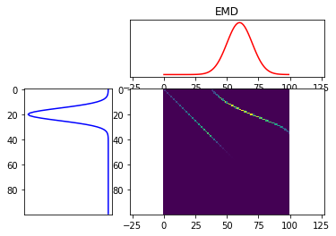
and the exact EMD solver used in PyEMD to give roughly the same number’s? What I mean is, (I think) the functions in the POT library return the transportation plan matrix T, and to get the actual wasserstein/EMD divergence, you calculate, the inner product,

<T,M> = trace(T'M) 

Where M is the ground metric matrix. But I get different numbers from both libraries, so I’m not sure which is right? I know you need to tune the regularization parameter lambda, but it should be easy to do that using downhill simplex/Nelder Mead

I want to get these test cases to reconcile - that way we’ve got something to check against when we try to code things, and do more complicated stuff in PyTorch. Otherwise, it’s too easy to make a mistake, without something solid to test against. :blush:

OK, sorry about this @tom :blush: , it seems the transport matrices from both PyEMD and POT do roughtly match - do want to check this?


import numpy as np
import matplotlib.pylab as pl
import pyemd 
import ot
from ot.datasets import get_1D_gauss as gauss

#%% parameters

n=100 # nb bins

# bin positions
x=np.arange(n,dtype=np.float64)

# Gaussian distributions
a=gauss(n,m=20,s=5) # m= mean, s= std
b=gauss(n,m=60,s=10)

# loss matrix
M=ot.dist(x.reshape((n,1)),x.reshape((n,1)))
M/=M.max()

#%% EMD with PyEMD library

div, T_pyemd = pyemd.emd_with_flow(a,b,M)
T_pyemd = np.array(T_pyemd)

#%% EMD with POT library

T_pot = ot.emd(a,b,M)

#%% Sinkhorn with POT library

lambd=1e-3
T_sink = ot.sinkhorn(a,b,M,lambd)

#%% plot each of the transport matrices

ot.plot.plot1D_mat(a,b,T_pyemd,'Exact OT matrix using PyEMD')
pl.show()

ot.plot.plot1D_mat(a,b,T_pot,'Exact OT matrix using POT')
pl.show()

ot.plot.plot1D_mat(a,b,T_sink,'Sinkhorn OT matrix using POT')
pl.show()

To compute the distance, you need to integrate:

dist=(M*T).sum()

Something seems to be up with pyemd, though: If you use your example but with larger stddev (e.g. 10 and 30), the “optimal” plan pyemd emits here clearly is broken (as the monotone transport function gives the optimal plan and I see two distinct areas)…

Hey thanks a lot for that! I think you’ve found something!

I do think PyEMD is a bit finicky, but the distances seem to be roughly the same,

>>> #%% EMD with PyEMD library
... 
>>> div_pyemd, T_pyemd = pyemd.emd_with_flow(a,b,M)
>>> T_pyemd = np.array(T_pyemd)
>>> div_pyemd
0.16684170730400028
>>> 
>>> #%% EMD with POT library
... 
>>> T_pot = ot.emd(a,b,M)
>>> div_pot_emd = np.trace( np.matmul( T_pot.transpose() , M) )
>>> div_pot_emd
0.16580581101906636

I guess then, we should go with the POT library, as that’s probably more reliable?

On another note, I think their choice of lambda=1e-3 is reasonable, I tried to tune it but it did’nt really make much difference,


#%% Use the downhill simplex method to find lambd
 
import numpy as np
from scipy.optimize import minimize

T_pot = ot.emd(a,b,M)
div_pot_emd = np.trace( np.matmul( T_pot.transpose() , M) )

#objective functon
def tune_lambda(x):
    #%% Sinkhorn approximate EMD using POT library
    T_sink = ot.sinkhorn(a,b,M,x)
    div_pot_sink = np.trace( np.matmul( T_sink.transpose() , M) )
    error = abs(div_pot_emd - div_pot_sink)
    return error

x0 = 1e-3 # initial guess

res = minimize(tune_lambda, x0, method='nelder-mead', options={'xtol': 1e-8, 'disp': True})

print(res.x)

Some speed tests for you @tom, only x10 at the moment?

It should be faster when i) it’s run on the gpu, ii) the histograms get bigger, iii) increase the dimensions, i.e images or higher dimension tensors, iv) tune lambda

Check out figure 4, from Marco Cuturi’s original paper,

#-----------------------------------------------------------------------------------------
#%% Speed Tests - see https://github.com/rflamary/POT/blob/master/examples/plot_OT_1D.py
#-----------------------------------------------------------------------------------------

import numpy as np
import pyemd 
import ot
import functools
from time import time
from ot.datasets import get_1D_gauss as gauss

#@functools.lru_cache (maxsize=None) # hash(tuple( yadda, yadda
def pyemd_linprog(n,a,b,M):
    start = time()
    for i in range(n): 
        div_pyemd = pyemd.emd(a,b,M)
    run_time = time() - start
    print(run_time)

#@functools.lru_cache (maxsize=None)
def pot_sinkhorn(n,a,b,M,lambd):
    start = time()
    for i in range(n): 
        T_sink = ot.sinkhorn(a,b,M, lambd)
        #div_pot_sink = np.trace( np.matmul( T_sink.transpose() , M) )
    run_time = time() - start
    print(run_time)

#%% parameters

n=128 # nb bins

# bin positions
x=np.arange(n,dtype=np.float64)

# Gaussian distributions
a=gauss(n,m=20,s=5) # m= mean, s= std
b=gauss(n,m=60,s=10)

# loss matrix
M=ot.dist(x.reshape((n,1)),x.reshape((n,1)))
M/=M.max()

##--------
runs=1000
lambd = 1

>>> pyemd_linprog( runs, a, b, M )
21.02236819267273
>>> pot_sinkhorn( runs, a, b, M, lambd )
2.0207273960113525

Hi @AjayTalati,

I started an implementation here: https://github.com/t-vi/pytorch-tvmisc/blob/master/wasserstein-distance/Pytorch_Wasserstein.ipynb

I’m not terribly impressed by the numerical stability, I’ll have to look into that.

Best regards

Thomas

1 Like

Hi @tom

Wow !!!

That’s pretty amazing how quickly you did that !!! Very, very impressive.

Let me go over it and try to do some testing - I need to get my slow old brain working :slight_smile: !! Be nice to do a test verses the unregularized version, i.e.

ot.lp.emd : Unregularized OT

So now that you have a Wasserstein loss that you can backprop through maybe you want to train a plain vanilla GAN with it, it would be interesting to see how it compares, here’s a quite basic version that’s new, and converges quite fast,

Be interesting if you could use your loss layer to improve it?

Perhaps you want to get in touch with Rémi Flamary, http://remi.flamary.com/, I’m sure he’ll be very impressed and be bursting with ideas for possible collaboration :smile:

Best regards,

Ajay

Hi Tom,

Yes as you said, I’m also getting a lot of Warning: numerical errrors numerical stability warnings?

Your implementations fine, (thanks once again for trying it), I’m guessing the problems simply the inherent instability of the different versions of the SK algorithm??

I’ve tried testing the linear programming ot.emd, against your implementation, and the numpy functions ot.bregman.sinkhorn_epsilon_scaling(a,b,M,1) etc. Like you showed the stabilized algorithm is much more stable than the vanilla version, although the relative rankings are still a little off?

So practically the task we want to address is not really can be reproduce the same values as the linear program emd algorithm. Rather we’re interested in ranking distributions.

To put it simply, if the linear program emd algorithm ranks, A and B, closer than A and C, then any approximate algorithm, (eg Sinkhorn-Knopp), should also give the same relative ranking.

I’m also trying it with discrete distributions, i.e. the histograms used in the original emd paper, but it works much better with Gaussians.

All the best,

Ajay